Epita:Algo:Course:Info-Sup:Trees Structures

A tree is a set of nodes storing elements in a parent-child relationship with different properties.

Binary trees

A binary tree is a recursive structure. It is either a null tree ( Ø ), or a tree that contains a root node and at most two subtrees ( < o, G, D > ) where o is the root node and L and R are two distinct subtrees (respectively left subtree and right subtree).

Figure 1. Graphical example of binary tree.

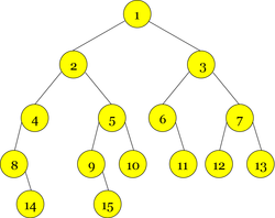
In this example, we have numbered each node to differentiate them. Something important to note is that a binary tree is not necessarily symmetric.

Remark: by convention, trees are drawn growing downwards.

Binary tree Algebraic Abstract Type

types

   binarytree

uses

   node, element


operations

   emptytree : $\rightarrow$ binarytree
     <_,_,_> : node x binarytree x binarytree $\rightarrow$ binarytree
        root : binarytree $\rightarrow$ node
           l : binarytree $\rightarrow$ binarytree
           r : binarytree $\rightarrow$ binarytree
     content : node $\rightarrow$ element

preconditions

   root(B) is-defined-iaoi B ≠ emptytree
   l(B) is-defined-iaoi B ≠ emptytree
   r(B) is-defined-iaoi B ≠ emptytree

axioms

   root (<r,L,R>)=r
   l(<r,L,R>)=L
   r(<r,L,R>)=R

with
   node r
   binarytree B,L,R

We can notice in blue the necessary operation to get the content of a node. This operation is necessary for a Labeled tree.

Terminology

The handling of binary trees requires the use of appropriate vocabulary. The main elements are:

let <r,L,R> be the binary tree B

• r is the root of B, with no parent node
• L is the left subtree of B
• R is the right subtree of B
• we call left child (right child) of the node n_i the root node of the left subtree (right subtree) of the tree rooted by n_i
• the link from a parent to a child is called directed-edge. If it is to the left child (right child), we call it the left link (right link)
• if a node n_j is the child of a node n_i, we say that n_i is the parent of n_j
• Two nodes that are children of the same parent are siblings
• A node n_i is an ancestor of a node n_j if it exists on the path from the root to node n_j (if n_i is either the parent of n_j or an ancestor of the parent of n_j).
• Conversely, we say that a node n_i is a descendant of a noden_j if n_j is the ancestor of n_i (if n_i is either the child of n_j or a descendant of the child of n_j).
• each node has at most two child nodes
• if a node has one left child (right child), it is a left (right) single internal node
• if a node has two children, it is a double internal node
• A node is an external node if it has no children. It is also called a leaf
• A path from the root to a leaf is called a branch
• A binary tree has as many branches as leaves
• the path obtained by following just the left links (right links) is called left edge (right edge) of B
  

Remarks: Unlike in real life, binary trees are not varieties of evergreens or deciduous. When I want to delete a leaf, I do. But the most amazing thing is that I create a (leaf) whenever I want. We also forget the notions of family and kinship.

Properties of binary trees

Now we will see operations on trees that calculate various measures and then determine the complexity of algorithms applied to them (the trees of course, what are we talking about ?).

These operations are the following :

• The size of a tree B is the number of nodes of this tree, which is defined by:

S(B)=	$\Bigg\{$	0	if B is a null tree (empty)
		1+S(l(B))+S(r(B))	otherwise

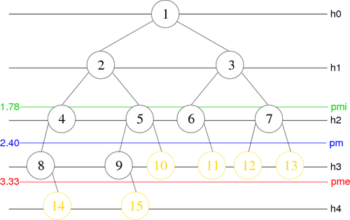
• The depth (level, height) of a node x of a tree B is the distance from the node to the root of the tree, it's defined by :

D(x)=	$\Bigg\{$	0	if x is the root of B
		1+D(y)	if y is the parent of x

• The height (order) of a tree B is the maximum depth of any node from the root. If a tree has only one node (the root), the height is zero. The height of an empty tree is not defined but could be considered as -1. The height of a tree B is specified by:

H(B) = max(H(x)) where x are the nodes of B

• The path Length (sum of the depth of all the nodes) of a tree B that is defined by:

PL(B) = ΣD(x) where x are all the nodes of B

• The external path length (sum of the depth of all the external nodes) of a tree B that is defined by:

EPL(B)=ΣD(xe) where xe are only the external nodes (leaves) of B

• The internal path length (sum of the depth of all the internal nodes) of a tree B that is defined by:

IPL(B)=ΣD(xi) where xi are only the internal nodes of B

then we have the following relation : PL(B)=EPL(B)+IPL(B)

• The average depth of a tree B that is defined by:

AD(B)=PL(B)/S(B)

• The external average depth of a tree B that is defined by:

EAD(B)=EPL(B)/Nbe where Nbe is the number of external nodes of B

• The internal average depth of a tree B that is defined by:

IAD(B)=IPL(B)/Nbi where Nbi is the number of internal nodes of B

Note : Measures like path length and average depth will be very useful to determine the complexity of algorithms applied to binary trees.

To clarify this, we will use the tree of Figure 1 and specify its characteristics and measurements. For this we will call this tree B and will retain the numbering of the nodes, which gives:

Figure 2. Some measures of the Figure 1 binary tree.

- 1 is the root of B, 2 is its left child and 3 its right child - siblings are : (2,3), (4,5), (6,7), (9,10), (12,13) - 1, 2, 3, 5 et 7 are "double" internal nodes of B - 4 is a "left single" internal node of B - 6, 8 and 9 are "right single" internal nodes of B - 10, 11, 12, 13, 14 and 15 are leaves of B - (1, 2, 4, 8) and (1, 3, 7, 13) are the left and right edges of B - (1, 2, 4, 8, 14), 1, 2, 5, 9, 15), (1, 2, 5, 10), (1, 3, 6, 11), (1, 3, 7, 12) and (1, 3, 7, 13) are branchs of B

- the nodes' depth of B are : 0 for node 1, 1 for nodes 2 and 3, 2 for nodes 4, 5, 6 and 7, 3 for nodes 8, 9, 10, 11, 12 and 13, 4 for nodes 14 and 15 - the height of B is H(B)=4 - the size of B is S(B)=15 - the sums of path length and average depths of B are : PL(B)=36, AD(B)=36/15 $\simeq$ 2,4, IPL(B)=16, IAD(B)=16/9 $\simeq$ 1,78, EPL(B)=20, EAD(B)=20/6 $\simeq$ 3,33

Particular binary trees

There are particular forms of binary trees. Knowing their specificities allow us to improve the algorithms on these trees using specific algorithms for their structure.

These trees are shown in figure 3 :

Figure 3. Particular binary trees.
Perfect	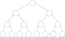Complete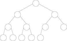
Full or proper	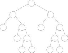Degenerate or filiform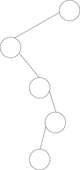

• A degenerate (filiform) tree is a tree in which for each parent node, there is only one associated child node. This means that in a performance measurement, the tree will behave like a linked list data structure.
• A perfect binary tree is a full binary tree in which all leaves are at the same depth or same level, and in which every parent has two children.(This is ambiguously also called a complete binary tree.)
• A complete binary tree is a binary tree in which every level, except possibly the last, is completely filled. At the deepest level, the height of the tree, all nodes are as far left as possible.
• A full (proper binary) binary tree is a tree in which every node has zero (the leaves) or two children. Sometimes a full tree is ambiguously defined as a perfect tree. There exist particular full binary trees which are called right (left) comb in which all left (right) child are leaves.

Note: This terminology often varies in the litterature, especially with the meaning of "complete" and "full".

Occurrence and hierarchical numbering

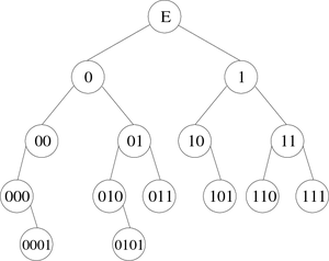
Another way to describe a binary tree is to attribute to each node a word constructed with "0" and "1". This word is named occurrence. By definition the root node is "E" and if a node has for occurrence "m", its left and right children have respectively the occurrences "m0" and "m1".

For the figure 1 tree called B, we would have:

B={E, 0, 1, 00, 01, 10, 11, 000, 010, 011, 101, 110, 111, 0001, 0101}

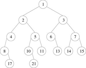
Binary trees can also be represented in breadth-first order. In this arrangement which is called hierarchical numbering, if a node is numbered i, its children are numbered 2 * i (for the left child) and 2 * i + 1 (for the right), while its parent is (if any) numbered i / 2 (assuming the root is numbered one).

For the example of figure 1 this would give :

Figure 4. Occurrence and hierarchical numbering representations of the binary tree of the figure 1.

Note: We will see later that the hierarchical numbering is very interesting on particular binary trees for an array implementation.

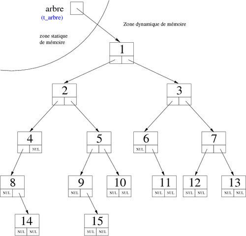
Implementations of binary trees

Like the elementary structures, we have the possibility to implement in memory the trees using dynamic or static representation. The latter may be used to simulate the former.

pointer-based implementation

This representation is virtually a layer of a binary tree. Each node contains an element (label) and two links: one to the left child and the other to the right child. It gives:

Types

   t_element = ...                /* Definition of element type */
   t_tree = $\uparrow$t_node               /* Definition of t_tree type (pointer on t_node) */
   t_node = record                /* Definition of t_node type */
      t_element elt
      t_tree   lc, rc
   end record t_node

Variables

   t_tree tree

This will give the following structure:

Figure 5. Pointer-based implementation of the binary tree in figure 1.

In this kind of implementation, the correspondences between the abstract operations and the pointer-based implementation (on a B binary tree) are the following:

Abstract type	⇔	Pointer-based implementation
B=emptytree		B=nul
B $\leftarrow$ < _, _, _>		Alloc(B)
root(B)		B$\uparrow$
l(B)		B$\uparrow$.lc
r(B)		B$\uparrow$.rc
Content(root(B))		B$\uparrow$.elt

Array implementation

In this representation, the tree will be contained in a vector (one-dimensional array) of records, each with three fields: the element and two integers (one for the left child and the other for the right child). The latter (both integers) referencing the vector index of the child concerned (am I clear enough?). The first index of the vector is 1, then we can use 0 as null pointer reference (the empty tree). We also need the position of the root given by an integer.

Note : When coded in C, it will then use -1, the base being 0.

Here is the declaration of such an algorithmic structure:

Constants

   MaxNb = 21

Types

   t_element = ...                     /* Definition of element type */
   t_node = record                     /* Definition of t_node type */
      t_element elt
      integer lc, rc
   end record t_node

   t_vectMaxNbnode = MaxNb t_node      /* Definition of t_node vector */
   t_tree = record                     /* Definition of t_tree type */
      t_vectMaxNbnode nodes
      integer         root
   end record t_tree

Variables

   t_tree tree

In this kind of implementation, the correspondences between the abstract operations and the array implementation (on a B binary tree) are the following:

Abstract type	⇔	Array implementation
B=emptytree		B.root=0
root(B)		B.root
l(B)		B.nodes[B.root].lc
r(B)		B.nodes[B.root].rc
Content(root(B))		B.nodes[B.root].elt

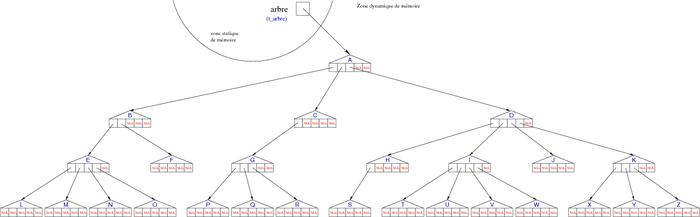
Adapted to the tree of Figure 1, we would have the table in Figure 6 (a). In fact, with this kind of tree, the root may be located in any index. So we can represent several trees at the same time in the same array, a forest for example. We just have to know for each tree where its root is.

Figure 6. Array implementation of a binary tree

elt fg fd 1 1 2 3 2 2 4 5 3 3 6 7 4 4 8 0 5 5 9 10 6 6 0 1 7 7 12 13 8 8 0 14 9 9 0 15 10 10 0 0 11 11 0 0 12 12 0 0 13 13 0 0 14 14 0 0 15 15 0 0 16 17 18 19 20 21		elt fg fd 1 1 2 3 2 2 4 5 3 3 6 7 4 4 8 0 5 5 10 11 6 6 0 13 7 7 14 15 8 8 0 17 9 10 9 0 19 11 10 0 0 12 13 11 0 0 14 12 0 0 15 13 0 0 16 17 14 0 0 18 19 20 21 15 0 0		elt 1 1 2 2 3 3 4 4 5 5 6 6 7 7 8 8 9 10 9 11 10 12 13 11 14 12 15 13 16 17 14 18 19 20 21 15
(a)		(b)		(c)

If we had used for the same tree, a hierarchical numbering nodes (not labels), we would have obtained this table Figure 6 (b).

This numbering has two major flaws:

• It forces us to fix the root of a non-empty tree to 1
• It generates holes in the table and therefore a relatively low occupancy rate.

That said, it is ideal for complete or perfect trees because all their levels, except the last, are filled, so no holes (Golfers of the World, Sorry).

In addition, the left child of a node ni is a node n2i and the right child is a node n2i+1, therefore we no longer need to reference the left and right children. This allows us to represent the tree using a simple vector of elements as shown in Figure 6 (c).

Remarks :

• We must find a way using the element to reference an empty tree (one possibility is to put the root at the 0 value).
• This representation allows us to know the father of a node without having to memorize it. For a node ni when i>1, this is the node n div 2.
• For a non-empty tree, the root must always be equal to 1.

For this representation (figure 6(c)), the algorithmic declaration would become:

Constants

   MaxNb = 21

Types

   t_element = ...                     /* Definition of element type */
   t_vectMaxNbnode = MaxNb t_element   /* Definition of t_node vector */
   t_tree = record                     /* Definition of type t_tree */
      t_vectMaxNbnode node
      integer         root
   end record t_arbre

Variables

   t_tree tree

In this case, the correspondences between the abstract operations and the array implementation would be the following:

Abstract type	⇔	Array implementation (hierarchical numbering)
B=emptylist		B.root=0
root(B)		B.root
l(B)		B.nodes[2*B.root]
r(B)		B.nodes[2*B.root+1]
Content(root(B))		B.nodes[B.root]

Traversals of a binary tree

A traversal of a tree is a systematic way of accessing, or "visiting," all the nodes of a tree.

There exist several ways to traverse a binary tree (you should be familiar with them):

• the depth-first traversal (Ooohh…).
• the breadth-first (level-order) traversal (aaaahh…)

The first examines the nodes as far down as possible in the tree (until a node has no children node) and the second processes all nodes of a tree by depth: first the root, then the children of the root, etc.

For the purpose of illustration, it is assumed that left nodes always have priority over right nodes. This ordering can be reversed as long as the same ordering is assumed for all traversal methods.

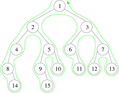
Depth-first traversal

This traversal is recursive by nature, it is used in maze solving algorithms (the "recursive backtracker" algorithm for example). Very simple: if you're at a wall (or an area you've already plotted), return failure, else if you're at the finish, return success, else recursively try moving in the four directions. Plot a line when you try a new direction, and erase a line when you return failure, and a single solution will be marked out when you hit success. When backtracking, it's best to mark the space with a special visited value, so you don't visit it again from a different direction. In Computer Science terms, this is basically a depth first search. This method will always find a solution if one exists, but it won't necessarily be the shortest solution. In French we call that kind of traversal le parcours profondeur main gauche.

Figure 8. Depth-first Traversal of a binary tree

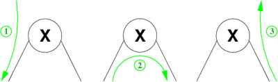
On the traversal of Figure 8, we have not accounted for the empty subtrees but they must be taken into account if one wants to admit that each node (including leaves) are met several times during the course. There are 3 orders induced by the depth-first traversal (see Figure 9) and are called:

• (1) Preorder visit each node before its children,
• (2) Inorder visit left subtree, node, right subtree,
• (3) Postorder visit each node after its children.

Figure 9. Orders induced by a Depth-first traversal of a binary tree

Depth-First traversal Algorithm

During this traversal, each node is met three times. We can assign to each of them a special processing. Furthermore, if we include the empty trees, we can also specify a special processing for them. It gives the following abstract algorithm that traverses a binary tree recursively:

Algorithm procedure depth-first_parse
Local parameters
   binarytree b
Begin
   if b=emptytree then
      /* end processing */
   else
      /* Preorder processing */
      depth-first_parse(l(b))
      /* Inorder processing */
      depth-first_parse(r(b))
      /* Postorder processing */
   endif
End algorithm procedure depth-first_parse

To clearly highlight the differences between the three orders induced by this traversal, we will replace them each time by the following display of the node:

Write(content(root(b))

If for each order we leave the other processes empty and then we apply this algorithm to the binary tree in Figure 8, we would obtain each time:

• (1) Preorder : 1, 2, 4, 8, 14, 5, 9, 15, 10, 3, 6, 11, 7, 12, 13

• (2) Inorder : 8, 14, 4, 2, 9, 15, 5, 10, 1, 6, 11, 3, 12, 7, 13

• (3) Postorder : 14, 8, 4, 15, 9, 10, 5, 2, 11, 6, 12, 13, 7, 3, 1

We note that depending on the type of traversal, the order of nodes differs.

Remarks :

• The hierarchical order, (1, 2, 3, 4, 5, 6, 7, 8, 9, 10, 11, 12, 13, 14, 15) for this example, is not visible because it corresponds to a breadth-first (level-order) traversal of the tree.
• All processes can be used at the same time to eventually achieve different things in a different order, or else because these processes are complementary. Thereafter, we will see the need to use several of these processes.

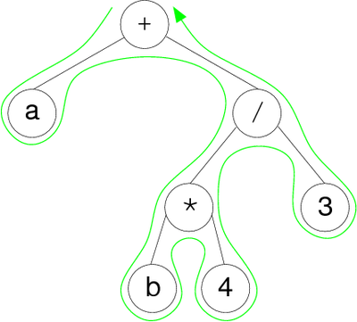
Depth-first traversal of a tree representing an arithmetical expression

We can use a binary tree to represent an arithmetical expression. In this case, the internal nodes store operators and the external nodes store operands. For the arithmetical expression ( a + ( ( b * 4 ) / 3 ) ), we can have the binary labeled tree of figure 10 :

Figure 10. arithmetical expression (a+((b*4)/3)

Remark: This expression uses only binary operators (with two operands), so it is a full (proper) binary tree.

For the tree of figure 10, the depth-first traversal, depending on orders, gives :

• (1) preorder : + a / * b 4 3
• (2) inorder  : a + b * 4 / 3
• (3) postorder: a b 4 * 3 / +

We note that the preorder and postorder are unambiguous. The first corresponding to the Polish notation and the second to the reverse Polish notation (rpn). This is unfortunately not the case for the inorder. Indeed, this series could correspond to different trees as shown in Figure 11.

Figure 11. Arithmetical expressions (a+((b*4)/3) et ((a+(b*4))/3)

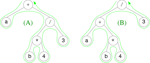
Indeed the Polish or reverse Polish notations are preceded or followed by operators of their operands. However for the inorder notation, we don't know if a + b * 4/3 corresponds to a + ((b * 4) / 3 or (a + (b * 4)) / 3. Actually this ambiguity can be easily resolved using parentheses to force the priority of operators.

It suffices to modify the depth-first traversal algorithm previously given as follows:

Algorithm procedure depth-first_inorder_parse
Local Parameters
   binarytree b
Begin
   if l(b)=emptytree and r(b)=emptytree then   /* b is a leaf */
      write(content(root(b)))                  /* End processing */
   else
      write('(')                               /* Preorder processing */
      depth-first_inorder_parse(l(b))
      write(content(root(b)))                  /* Inorder processing */
      depth-first_inorder_parse(r(b))
      write(')')                               /* Postorder processing */
   endif
End algorithm procedure depth-first_inorder_parse

That gives for trees given in Figure 11 the two following unambiguous series :

• Figure 11(A) : ( a + ( ( b * 4 ) / 3 ) )
• Figure 11(B) : ( ( a + ( b * 4 ) ) / 3 )

Remark : In the previous algorithm, we could change the test that checks whether the node where we are is a leaf. To do this, it suffices to create an extension to the Binary tree abstract type creating a new operation as follows:

operations

   leaf : binarytree $\rightarrow$ boolean

axioms

   b$\neq$emptytree & l(b)=emptytree & r(b)=emptytree $\Rightarrow$ leaf(b)=true 

Then the beginning of the algorithm will be :

Algorithm procedure depth-first_inorder_parse
Local Parameters
   binarytree b
Begin
   if leaf(b) then   /* b is a leaf */

Breadth-first (level-order) traversal

The traversal begins at a root node and inspects all the children nodes. Then for each of those children nodes in turn, it inspects their children nodes, and so on.

Remark : This traversal, also called level-order, is iterative by nature.

The Breadth-first traversal uses a Queue to memorize the two children of each node visited. That allows, at the next level, to retrieve them in the meet order. It gives the following algorithm :

Algorithm procedure breadth-first_parse
Local parameters
   binarytree b
Variables
   integer i
   queue q                              /* f memorizes the trees */
Begin
   q $\leftarrow$ emptyqueue
   q $\leftarrow$ enqueue(b,q)                    /* push of the b tree */
   while not(isempty(q)) do
      b $\leftarrow$ first(q)                     /* recover the 1st tree memorized */
      q $\leftarrow$ dequeue(q)                   /* remove this tree of the queue */
      write(content(root(b)))           /* display the root node of the recovered tree */
      if l(b))<>emptytree then
         q $\leftarrow$ enqueue(l(b),q)           /* push of the left subtree of b */
      endif
      if r(b))<>emptytree then
         q $\leftarrow$ enqueue(r(b),q)           /* push of the right subtree of b */
      endif
   endwhile
End Algorithm procedure breadth-first_parse

If we apply this algorithm to the binary tree in Figure 8, we would obtain:

1, 2, 3, 4, 5, 6, 7, 8, 9, 10, 11, 12, 13, 14, 15

Remarks :

• This algorithm performs the breadth-first traversal of any non-empty binary tree.
• Complexity is the same as the depth-first traversal.

General trees

A tree or general tree is a tree structure where the number of children is not limited to two. The recursive definition of a general tree is A = < o,A₁,...,A_n > where o is the root of A and A₁,...,A_n is a finite list, possibly empty (if n = 0), of disjointed trees. This list is called a forest. We obtain a tree by adding a root to a forest.

Figure 12. Graphical example of a tree.

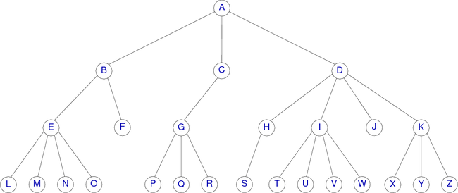
General tree Algebraic Abstract Type

types

   tree, forest

use

   node, integer, element


operations

         cons : node x forest $\rightarrow$ tree
         root : tree $\rightarrow$ node
     treelist : tree $\rightarrow$ forest
  emptyforest : $\rightarrow$ forest
       insert : forest x integer x tree $\rightarrow$ forest
       delete : forest x integer $\rightarrow$ forest
          nth : forest x integer $\rightarrow$ tree
      nbtrees : forest $\rightarrow$ integer
     content : node $\rightarrow$ element

preconditions

   insert(f,i,t) is-defined-iaoi 1 ≤ i ≤ 1 + nbtrees(f)
   delete(f,i) is-defined-iaoi f ≠ emptyforest & 1 ≤ i ≤ nbtrees(f)
   nth(f,i) is-defined-iaoi f ≠ emptyforest & 1 ≤ i ≤ nbtrees(f)

axioms

   root(cons(o,f))=o
   treelist(cons(o,f))=f
   nbtrees(emptyforest)=0
   nbtrees(insert(f,i,t))=nbtrees(f) + 1
   nbtrees(delete(f,i))=nbtrees(f) - 1
   1 ≤ i < k $\Rightarrow$ nth(insert(f,k,t),i) = nth(f,i)
   k = i $\Rightarrow$ nth(insert(f,k,t),i) = t
   k < i ≤ nbtrees(f)+1 $\Rightarrow$ nth(insert(f,k,t),i) = nth(f,i-1)
   1 ≤ i < k $\Rightarrow$ nth(delete(f,k),i) = nth(f,i)
   k ≤ i ≤ nbtrees(f)-1 $\Rightarrow$ nth(delete(f,k),i) = nth(f,i+1)

with
   node o
   tree t
   forest f
   integer i,k

Remarks :

• The "left-right" notion necessary to the binary tree disappears. That said, the vocabulary used for the general trees remains the same except for everything that uses this notion (of generality). For instance we no longer talk about a left or a right child, but about first child, second child and so on and a last child.
• The measurements on the trees are retained (height, path length, size, etc).

Implementations of general trees

There are several kinds of representations of general trees. The most intuitive are the linked-list and the n-tuple representations. Another one, very used, is the leftmost child-right sibling representation (a binary tree).

Vector-based (Array) implementation of general trees

In this case, the set of nodes is represented in a one-dimensional array (vector), oversized to allow us to add nodes if necessary. Each element is a record that contains the label of the node plus a pointer to its children list. The children list consists of records containing two fields : a pointer to a table element and another pointer to the next record (as for graph lists of adjacency). In this case, the algorithmic description would be:

Constants

   MaxNb = 27

Types

   t_element = ...                /* Definition of element type */
   t_pchild = $\uparrow$t_child            /* Definition of child node pointer (list) */

   t_node = record                /* Definition of type t_node */
      t_element  elt
      t_pchild   firstchild
   end record t_node

   t_child = record               /* Definition of type t_child */
      integer    childnodenumber
      t_pchild   nextchild
   end record t_child

   t_tree = MaxNb t_node         /* Definition of type y_tree (array) */

Variables

   t_tree tree

For the tree of figure 12, this would give :

Figure 13. Vector-based implementation of the general tree of figure 12.

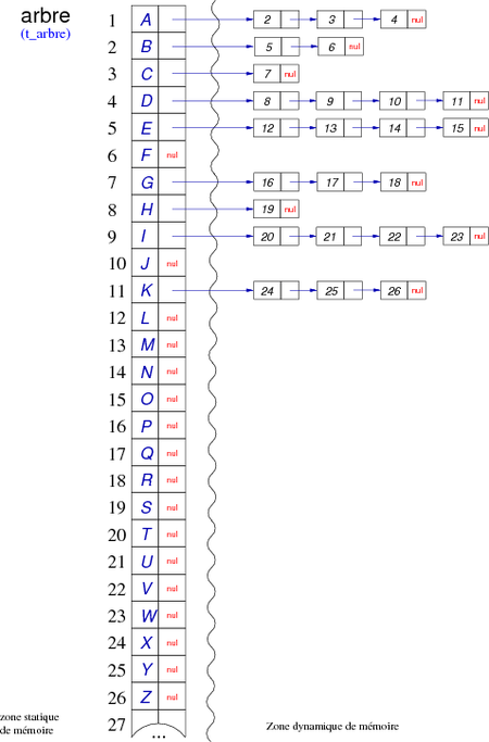
Linked-list (pointer) implementation of general trees

Remark : One possibility is to transform this representation to a full dynamic one replacing the vector by a linked list. In this case, nodes are interconnected by a dynamic link (pointer), and thereby in the record t_child the integer childnodenumber (index of the node in the table) is replaced by a pointer to the node address.

That gives the following algorithmic declaration :

Types

   t_element = ...                      /* Definition of element type */
   t_pnode = $\uparrow$t_node                    /* Definition of t_pnode (pointer to t_node)*/
   t_pchild = $\uparrow$t_child                  /* Definition of t_pchild (pointer to t_child) */

   t_node = record                      /* Definition of t_node */
      t_element elt
      t_pnode   nextnode, prevnode
      t_pchild  firstchild
   end record t_node

   t_child = record                     /* Definition of t_child */
      t_pnode   childnode               /* pointer to childnode */
      t_pchild  nextchild               /* pointer to next childnode */
   end record t_child

   t_tree = t_pnode                     /* Definition of t_tree (pointer to node) */

Variables

   t_tree tree

To visualize this structure, it is sufficient to see the adjacency list representation of graphs with a dynamic set of vertices.

Binary trees implementation (left most child-right sibling representation)

The way of representing general trees as binary trees is to use the left link as the left most child and the right link as the next sibling. This representation has several advantages:

• This is a bijective representation : One node in the general tree, one node in the binary tree.
• We can use the algorithms on binary trees (traversal, insertion of node, etc.), that are very simple to implement.

Remark : It seems obvious that this is the pointer-based implementation of a binary tree that is chosen.

The algorithmic description would be:

Types

   t_element = ...                /* Definition of element type */
   t_tree = $\uparrow$t_node               /* Definition of t_tree (pointer to t_node) */
   t_node = record                /* Definition of t_node */
      t_element elt
      t_tree    leftmostchild, rightsibling
   end record t_node

Variables

   t_tree tree

For the tree of figure 12, this would give :

Figure 15. left most child-right sibling representation of the tree of figure 12.

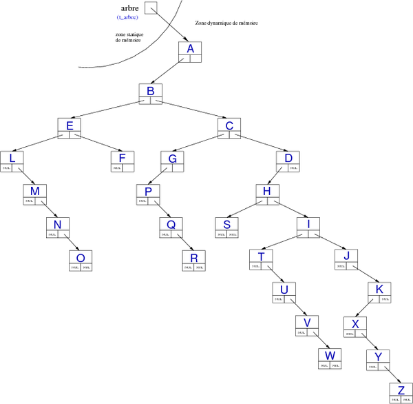
Working with this tree is very simple. For example to find the child of a node (in the general tree), it is sufficient from its right child (in the binary tree) to traverse the right edge (always in the binary tree). Similarly, calculating the height of the tree can easily be done in the binary tree by considering only the height of the left child (the first child in the general tree) and not the right siblings (which are located at the same height).

Remarks :

• The corresponding binary tree is not balanced at all.
• The preorder and inorder traversals of the corresponding binary tree will give the same encountering order of nodes as those given by the respectively preorder and postorder traversals of the implemented general tree.

N-tuple representation

If you know the maximum number of children that can have a node, it is possible to represent the tree as N-tuple. This representation is an extension of the dynamic representation of binary trees. Here, the number of children is not two, but one that we have specified (using a constant). Assuming there are five maximum children, the algorithmic declaration would be the following:

Constants

   MaxChildrenNb = 5                     /* Maximum number of children */

Types

   t_element = ...                       /* Definition of element type */
   t_tree = $\uparrow$t_node                      /* Definition of t_tree  (pointer to t_node) */
   t_childrentab = MaxChildrenNb t_tree  /* Definition of children vector */

   t_node = record                       /* Definition of t_node */
      t_element     elt
      t_childrentab children
   end record t_node

Variables

   t_tree tree

For the tree of figure 12, this would give :

Figure 16. n-tuple tree representation of the tree of figure 12.

Traversals of a general tree

As for a binary tree the traversal of a tree is a systematic way of accessing, or "visiting," all the nodes of the tree.

There exist several ways to traverse a tree (you should be familiar with them):

• the depth-first traversal (Ooohh…).
• the breadth-first (level-order) traversal (aaaahh…)

The first (recursive by nature) examines the nodes as far down as possible in the tree (until a node has a no children node) and the second (iterative by nature) processes all nodes of a tree by depth: first the root, then the children of the root, etc.

Depth-first traversal

To traverse a general tree, we can use the same principle as the depth-first traversal of binary trees. The difference lies in the fact that there only two induced orders : there is no inorder traversal, but an intermediate process at each passage of one child to another. In other words, a node is met one time more than its number of children: once before visiting its first child (preorder), once between each child and its right sibling and once when returning from the last child (postorder).

The algorithm used for this traversal is that of the binary tree "slightly modified". Indeed, processes have to be placed inside a loop whose number of iterations depends on the subtree number of the tree that we have to traverse.

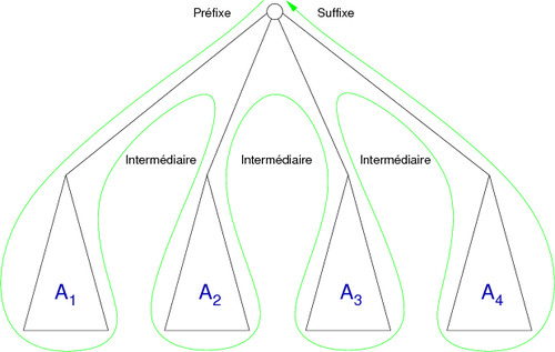
To illustrate this, assume a general tree A = <o, A1, A2, A3, A4>, we get the path of Figure 17 (resembling nothing so much as an x-ray of the hand of Mickey highlighting the presence of an exo-skeleton :D):

Figure 17. Depth-first traversal of a general tree.

More seriously, it can be seen on this traversal that the root node is visited five times, once when descending toward A1 (preorder process), three times from A1 to A2, A2 to A3 and A3 to A4 (intermediate processes), and finally when returning from A4 (postorder process).

It gives the following abstract depth-first traversal of a tree:

Algorithm procedure depth-first_parse
Local parameters
   tree t
Variables
   integer i, childnb
Begin
   childnb $\leftarrow$ nbtrees(treelist(t)) 
   if leaf(t) then                    /* t is a leaf (childnb=0) */
      /* End processing */
   else
      /* Preorder processing */
      for i $\leftarrow$ 1 to childnb-1 do
         depth-first_parse(nth(treelist(t),i))
         /* Intermediate processing */
      endfor
      depth-first_parse(nth(treelist(t),childnb))
      /* Postorder processing */
   endif
End algorithm procedure depth-first_parse

Remarks :

• We use an additional operation presented with the binary tree abstract data type that is the leaf. This operation should of course be defined as an additional operation of the general tree abstract data type.
• The number of possible treatments of a node is not limited to three, but may actually be equal to the number of children plus one. Indeed, the number of intermediate processes depends on the value of the loop index and therefore allows for a particular treatment each time.

For example, using the general tree of Figure 12, we can list the nodes as follows:

(A(B(E(L)(M)(N)(O))(F))(C(G(P)(Q)(R)))(D(H(S))(I(T)(U)(V)(W))(J)(K(X)(Y)(Z))))

using the following algorithm :

Algorithm procedure depth-first_parse_lisp
Local parameters
   tree t
Variables
   integer i, childnb
Begin
   childnb $\leftarrow$ nbtrees(treelist(t)) 
   if leaf(t) then                        /* t is a leaf (childnb=0) */
      write('(',content(root(t)),')')
   else
      write('(',content(root(t)))
      for i $\leftarrow$ 1 to childnb-1 do
         depth-first_parse_lisp(nth(treelist(t),i))
      endfor
      depth-first_parse_lisp(nth(treelist(t),childnb))
      write(')')
   endif
End algorithm procedure depth-first_parse_lisp

that could be optimized in the following way :

Algorithm procedure depth-first_parse_lisp
Local parameters
   tree t
Variables
   integer i, childnb
Begin
   childnb $\leftarrow$ nbtrees(treelist(t)) 
   write('(',content(root(t)))
   if not(leaf(t)) then                        /* t is not a leaf (childnb>0) */
      for i $\leftarrow$ 1 to childnb-1 do
         depth-first_parse_lisp(nth(treelist(t),i))
      endfor
      depth-first_parse_lisp(nth(treelist(t),childnb))
   endif
   write(')')
End algorithm procedure depth-first_parse_lisp

Breadth-first traversal

The traversal begins at a root node and inspects all the children nodes. Then for each of those children nodes in turn, it inspects their children nodes, and so on.

Actually the traversal is done by distance (level, depth or height in this case), that is to say that we first scan all the nodes at a distance of 1 from the root, then all those that are located at a distance of 2 and so on ...

Remark : This traversal, also called level-order, is iterative by nature.

The Breadth-first traversal uses a Queue to memorize all the children of each node visited. That allows, at the next level, to retrieve them in the meet order. It gives the following algorithm :

Algorithm procedure breadth-first_parse
Local parameters
   tree t
Variables
   integer i
   queue q                                        /* f stocke les arbres */
Begin
   q $\leftarrow$ emptyqueue
   q $\leftarrow$ enqueue(q,t)                              /* storage of the tree */
   while not(isempty(q)) do
      t $\leftarrow$ first(f)                                /* recovery of the first tree stored */
      q $\leftarrow$ dequeue(q)                             /* release the tree of the queue */
      write(content(root(t)))                     /* displaying the content of the root node of the recovered tree*/
      for i $\leftarrow$ 1 to nbtrees(treelist(t)) do
         q $\leftarrow$ enqueue(q,nth(treelist(t),i)))      /* storage of the ith subtree of t */
      endfor
   endwhile
End algorithm procedure breadth-first_parse

Using the general tree of Figure 12, we can list the nodes as follow:

A, B, C, D, E, F, G, H, I, J, K, L, M, N, O, P, Q, R, S, T, U, V, W, X, Y, Z

Remark : Complexity is the same as the depth-first traversal.

---

(Christophe "krisboul" Boullay)