Epita:Algo:Course:Sup-Info:Elementary Data Structures

The linear list

The linear list is the most fundamental abstract data type that can be found. They are sequences of elements. The order of elements in a list doesn't depend on the element values, but on their position in the list. There are two ways to describe a list : iteratively or recursively. We will consider both and see what kind of memory implementation is best suited for these different types of list. Lists are a particularly flexible structure because they can grow and shrink on demand, and elements can be accessed, inserted, modified and deleted at any position within a list. Lists can also (for the same price:)) be concatenated together, split into sublists, used to retrieve information, and so on.

The recursive list type

types

   list, box

uses

   element

operations

   emptylist : $\rightarrow$ list
        cons : list x element $\rightarrow$ list
        tail : list $\rightarrow$ list
        head : list $\rightarrow$ box
    contents : box $\rightarrow$ element
       first : list $\rightarrow$ element
        next : box $\rightarrow$ box

preconditions

   tail(l) is-defined-iaoi l ≠ emptylist
   head(l) is-defined-iaoi l ≠ emptylist
   first(l) is-defined-iaoi l ≠ emptylist

axioms

   first(l) = contents(head(l))
   tail(cons(e,l)) = l
   first(cons(e,l)) = e
   next(head(l)) = head(tail(l))

with

   list l
   element e

Thereafter we won't give terminology elements used in abstract type definitions. So, for the last time, in the above abstract type we have:

• List and Box as defined types
• element as predefined types
• head and next as internal operations of Box
• contents as observer of Box
• emptylist, tail and cons as internal operations of list
• first as observer of list

These operations are not defined everywhere, therefore there are preconditions. The algebraic definition gives to the various functions the following roles:

• emptylist create a list without element (a kind of "constructor")
• head retrieves the first box
• contents retrieves the element which is inside a box
• first retrieves the first element of a list (without using intermediate box )
• tail deletes the head element and retrieves the rest of the list
• cons creates an element at the first position (inserting it in a new box just before the existing list)
• next pass to the next box

The iterative list type

types

   list, box

uses

   integer, element

operations

   emptylist : $\rightarrow$ list
      access : list x integer $\rightarrow$ box
    contents : box $\rightarrow$ element
         nth : list x integer $\rightarrow$ element
      length : list $\rightarrow$ integer
      delete : list x integer $\rightarrow$ list
      insert : liste x integer x element $\rightarrow$ list
        next : box $\rightarrow$ box

preconditions

   access(l,k) is-defined-iaoi l ≠ emptylist & 1 ≤ k ≤ length(l)
   delete(l,k) is-defined-iaoi l ≠ emptylist & 1 ≤ k ≤ length(l)
   insert(l,k,e) is-defined-iaoi 1 ≤ k ≤ length(l)+1

axioms

   length(emptylist) = 0
   length(delete(l,k)) = length(l)-1
   length(insert(l,k,e)) = length(l)+1

   1 ≤ i < k $\Rightarrow$ nth(delete(l,k),i) = nth(l,i)
   k ≤ i ≤ length(l)-1 $\Rightarrow$ nth(delete(l,k),i) = nth(l,i+1)

   1 ≤ i < k $\Rightarrow$ nth(insert(l,k,e),i) = nth(l,i)
   k = i $\Rightarrow$ nth(insert(l,k,e),i) = e
   k < i ≤ length(l)+1 $\Rightarrow$ nth(insert(l,k,e),i) = nth(l,i-1)

   contents(access(l,k)) = nth(l,k)
   next(access(l,k)) = access(l,k+1)

with
   list l
   integer i,k
   element e

This presentation is another form of implementation of linear lists. In fact, the basic operation is no longer the access to the first box of a list (head operation), but the operation access which refers to the k^th place of this list. Other operations directly arise from this operation.

The iterative list abstract type, although more adapted to other functionings, can also describe recursive processing.

What is important is to understand is that we are in fact describing the same data, only their manipulations are different. A simple way to demonstrate this is to write a type of operation in terms of the other and vice versa.

To start, we are going to write the operations of the recursive type using the operations of the iterative type:

recursive	⇔	iterative
head (l)		access (l,1)
first (l)		nth (l,1)
tail (l)		delete (l,1)
cons (e,l)		insert (l,1,e)

And inversely:

iterative	⇔	recursive
insert (l,i,e)		l2 $\leftarrow$ emptylist
(i-1) times	$\Bigg\{$	l2 $\leftarrow$ cons (first (l),l2)
		l $\leftarrow$ tail (l)
		l $\leftarrow$ cons (e,l)
(i-1) times	$\Bigg\{$	l $\leftarrow$ cons (first (l2),l)
		l2 $\leftarrow$ tail (l2)

As can be seen, the match in this case is not just a single operation but, the operation insert has been transcribed using only the operations of the recursive list.

Note: The translation of the other operations has been left in exercices.

Additional operations on list type

Of course, we often need additional operations on lists such as concatenation of two lists or the search for an item in a list. We call them : additional operations on the defined type. There is no need to represent the abstract type which is assumed to be known (I hope!).

For these two additional operations, we will present the profile, preconditions if necessary, and axioms for iterative and recursive lists.

Concatenation of two lists

The concatenation (also called append) of two lists is the operation of joining two lists end-to-end. The elements of the 2^nd list are added to the end of the first (elements keep their own place within each list).

operations

   append : list x list $\rightarrow$ list

axioms (recursive list)

   append(emptylist,l) = l
   append(cons(e,l),l2) = cons(e,append(l,l2))

axioms (iterative list)

   length(append(l,l2)) = length(l)+length(l2)
   1 < i < length(l) $\Rightarrow$ nth(append(l,l2),i) = nth(l,i)
   length(l)+1 < i < length(l)+length(l2)
      $\Rightarrow$ nth(append(l,l2),i) = nth(l2,i-length(l))

with

   list l,l2
   integer i
   element e

Search for an element

The research consists in finding an item in a list and returning its position if this element exists in the list. The problem is that the research is not defined for a non-present element. Therefore a research precondition is necessary. We will describe it using an auxiliary operation ispresent.

operations

    research : element x list $\rightarrow$ box
   ispresent : element x list $\rightarrow$ boolean

preconditions

   research(e,l) is-defined-iaoi ispresent(e,l) = true

axioms (recursive list)

   ispresent(e,emptylist) = false
   e = e2 $\Rightarrow$ ispresent(e2,cons(e,l)) = true
   e ≠ e2 $\Rightarrow$ ispresent(e2,cons(e,l)) = ispresent(e2,l)
   ispresent(e,l) = true $\Rightarrow$ contents(research(e,l)) = e

axioms (iterative list)

   ispresent(e,emptylist) = false
   e = e2 $\Rightarrow$ ispresent(e2,insert(l,i,e)) = true
   e ≠ e2 $\Rightarrow$ ispresent(e2,insert(l,i,e)) = ispresent(e2,l)
   ispresent(e,l) = true $\Rightarrow$ contents(research(e,l)) = e

with

   list l
   integer i
   element e,e2

Implementation of Lists

Lists, as all other data types, are implementable in different ways. The two basic forms are array implementation (static representation) and linked list implementation (dynamic representation using pointers).

Of course, for sophisticated data types, it is possible to represent them by a hybrid implementation (static and dynamic).

Array Implementation of Lists

Example of algorithmic declaration :

Constants

   Maxnb = 20

Types

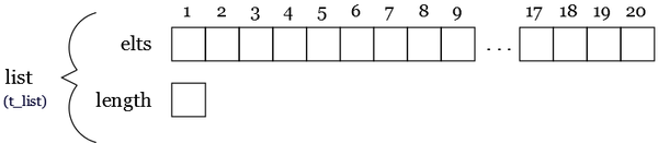
   t_element = ...                     /* Element Definition */
   t_vectMaxNbelts = Maxnb t_element   /* Array of elements Definition */
   t_list = record                     /* List Definition */
      t_vectNbmaxelts elts
      integer length
   end record t_list

Variables

   t_list list

This could correspond to the following structure:

In the array Implementation, we define the type t_list as a record having two fields. The first is an array of t_element whose length (Maxnb) is sufficient to hold the maximum size list that will be encountered. The second field is an integer (length) indicating the position of the last list element in the array. Indeed, the array implementation requires us to specify the maximum size of a list, then the field length indicates how many elements are really used in the array. The i^th element of the list is in the i^th cell of the array. Positions in the list are represented by integers, the i^th position by the integer i. It's very simple (a 5 year-old would understand. At least, I think ...).

Remark 1: Inserting an element into the middle of the list requires shifting all following elements one place over in the array to make room for the new element. Similarly, deleting any element except the last also requires shifting elements to close up the gap. This is what makes this representation inefficient in case of frequent modifications of elements.

Remark 2: Contrary to what you might think, this representation is perfectly suited for recursive lists. In this case, the length serves as first position (Head box).

Pointer implementation of Lists

Example of Algorithmic declaration :

Types

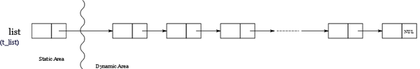
   t_element = ...         /* Element definition */
   t_plist = $\uparrow$t_liste      /* pointeur t_plist definition */
   t_list = record         /* type t_list definition */
      t_element elt
      t_plist lien
   end record t_list

Variables

   t_plist list

This could correspond to the following structure:

The NUL pointer represents the end of the list (emptylist).

The pointer implementation uses only as much space as is needed for the elements currently on the list. This implementation of lists uses pointers to link successive list elements. It frees us from using contiguous memory for storing a list and hence from shifting elements to make room for new elements or to close up a gap created by delete elements. But one price we pay for this liberty is extra space for the pointer in each cell.

Remark: The major drawback is not being able to access the K^th element directly. Indeed, in this kind of implementation, we have to follow the link cell by cell until locate the searched element. However, it is easy to concatenate two lists, add, or delete an item without having to shift any element. It is also very well suited to recursive processing.

Implementation variants of lists

Using a sentinel

In some implementations, an extra sentinel or dummy node may be added before the first data record and/or after the last one. This convention simplifies and accelerates some list-handling algorithms, by ensuring that all links can be safely dereferenced and that every list (even one that contains no data elements) always has a "first" and "last" node.

In this case, the variable declaration becomes:

Variables

   t_list list

If we add a sentinel before the first cell, we could have the following structure:

Circular Lists

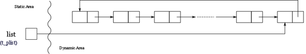
In the last node of a list, the link field often contains a null reference, a special value used to indicate the lack of further nodes. A less common convention is to make it point to the first node of the list. In that case the list is said to be circular or circularly linked, otherwise it is said to be open or linear. If we've got a one element list, this one links itself.

In this case, there's no declaration type modification and we could have the following structure

Note : We could also use a sentinel (a node) instead of a single pointer

Doubly-Linked Lists

In a number of applications we may wish to traverse a list both forwards and backwards efficiently. Or, given an element, we may wish to determine the preceding and following elements quickly. In such situations we might wish to give each cell on a list a pointer to both the next and previous cells on the list.

In a doubly linked list, each node contains, besides the next-node link, a second link field pointing to the previous node in the sequence. The two links may be called forward(s) and backwards, or next and prev(ious).

In this case, the variable declaration becomes:

Types

   t_element = ...             /* Element Definition */
   t_penreg = $\uparrow$t_enreg         /* Pointer t_penreg Definition */
   t_enreg = record            /* t_enreg Definition */
      t_element elt
      t_penreg next,prev
   end record t_enreg
   t_list = record             /* t_liste Définition*/
      t_penreg first,last
   end record t_list

Variables

   t_list list

it could correspond to the following structure:

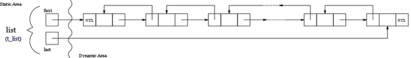
Of course, it is always possible to build other structures, for example a circular doubly linked list.

To conclude on the possible variants of the implementations of lists, it's possible to simulate pointers with cursors, that is, with integers that indicate positions in arrays. In this case, the array elements are records with two fields: the element and an integer that is used as a cursor.

In fact almost everything is possible, but using this kind of structure has no interest because it has all the drawbacks of static and dynamic combined (a bit like the Side-Car).

Stacks and Queues

Stacks

Stacks are LIFO (Last In First Out) structures. That is to say that a stack is a special kind of list in which all inputs (insertions) and outputs (deletions) take place at one end, called the top. The intuitive model of a stack is a pile of poker chips on a table, books on the floor, or dishes on a shelf where, if you are "normal" (and for some of students it's not sure), it is only convenient to remove the top object on the pile or add a new one above the top. In other words, it's a collection of items from which only the most recently added item may be removed.

The algebraic abstract data type Stack is the following:

types

   stack

uses

   boolean, element

operations

   emptystack : $\rightarrow$ stack
         push : stack x element $\rightarrow$ stack
          pop : stack $\rightarrow$ stack
          top : stack $\rightarrow$ element
      isempty : stack $\rightarrow$ boolean

preconditions

   pop(p) is-defined-iaoi isempty(p) = False
   top(p) is-defined-iaoi isempty(p) = False

axioms

   pop(push(p,e)) = p
   top(push(p,e)) = e
   isempty(emptystack) = True
   isempty(push(p,e)) = False

with

      stack p
    element e

The algebraic definition gives to the various functions the following roles:

• emptystack creates a stack without element (a kind of "constructor")
• push inserts an element at the top of a stack
• pop deletes the top element of a stack
• top retrieves the element at the top of a stack
• isempty returns true if and only if the stack is empty

Array Implementation of Stacks

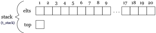
The array-based implementation of lists we gave before is not a particularly good one for stacks, as every push or pop requires moving the entire list up or down, thus taking time proportional to the number of elements on the stack. A better arrangement for using an array takes account of the fact that insertions and deletions occur only at the top. We can anchor the bottom of the stack at the bottom (low-indexed end) of the array, and let the stack grow towards the top (high-indexed end) of the array. A integer cursor called top indicates the current position of the first stack element.

Example of algorithmic declaration :

Constantes

   Nbmax = 20                         /* Maximum number of elements in the stack */

Types

   t_element = ...                    /* Element definition */
   t_elements = Nbmax t_element       /* Element array definition  */
   t_stack = record                   /* Stack type definition */
      t_elements elts
      integer top
   end record t_stack

Variables

   t_stack stack

This idea is shown in the following figure :

Linked-link representation of stacks

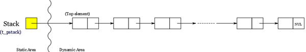
The linked-list representation of a stack is easy, as push and pop operate only on the header cell and the first cell on the list. It may be noted that the link is a previous link. When it pops, this link allows us to know what element, if it exists, had previously been stacked.

Example of Algorithmics declaration :

Types

   t_element = ...                   /* Element Definition */
   t_pstack = $\uparrow$t_stack               /* Pointer Type Definition */
   t_stack = record                  /* Définition du type t_pile */
      t_element elt
      t_pstack  previous
   end record t_stack

Variables

   t_pstack stack

This idea is shown in the following figure :

Queues

Queues are another special kind of list, where items in the collection are kept in order. They are inserted at one end (the rear) and deleted or removed at the other end (the front). Another name of Queue is a FIFO (First In First Out) list. In a FIFO data structure, the first element added to the queue will be the first one to be removed. This is equivalent to the requirement that once an element is added, all elements that were added before have to be removed before the new element can be invoked.

The intuitive model of a Queue is a people queue in front of a theater.

Queues provide services in computer science, transport, and operations research where various entities such as data, objects, persons, or events are stored and held to be processed later. In these contexts, the queue performs the function of a buffer.

The algebraic abstract data type Queue is the following:

types

   queue

uses

   boolean, element

operations

   emptyqueue : $\rightarrow$ queue
      enqueue : queue x element $\rightarrow$ queue
      dequeue : queue $\rightarrow$ queue
        front : queue $\rightarrow$ element
      isempty : queue $\rightarrow$ boolean

preconditions

   dequeue(q) is-defined-iaoi isempty(q) = False
   front(q) is-defined-iaoi isempty(q) = False

axioms

   isempty(q) = true $\Rightarrow$ front(enqueue(q,e)) = e
   isempty(q) = false $\Rightarrow$ front(enqueue(q,e)) = front(q)
   isempty(q) = true $\Rightarrow$ dequeue(enqueue(q,e)) = emptyqueue
   isempty(q) = false $\Rightarrow$ dequeue(enqueue(q,e)) = enqueue(dequeue(q),e)
   isempty(emptyqueue) = true
   isempty(enqueue(q,e)) = false
 
with

      queue q
    element e

The algebraic definition gives to the various functions the following roles:

• emptyqueue creates a queue without element (a kind of "constructor")
• enqueue inserts an element at the end of a queue
• dequeue deletes the front element (the first element of the queue)
• front retrieves the first element of a queue
• isempty returns true if and only if the queue is empty

Array implementation of queues

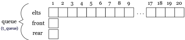
We need an array to store the elements and two integers Front and Rear that allow us to always know where the beginning and the end of the Queue are.

Example of algorithmics declaration:

Constants

   Nbmax = 8                          /* Maximum number of elements in the queue */

Types

   t_element = ...                    /* Element type definition */
   t_elements = Nbmax t_element       /* Elements array definition */
   t_queue = record                   /* Queue type definition */
      t_elements elts
      integer font,rear
   end record t_queue

Variables

   t_queue queue

it could correspond to the following structure:

But this representation is not very efficient. Indeed, Dequeue, which removes the first element, requires the entire queue be moved up one position in the array. Thus Dequeue takes ω(n) times if the queue has n elements.

To avoid this expense, we must take a different viewpoint. Think of an array as a circle, where the first position follows the last as suggested in the next figure. The queue is found somewhere around the circle in consecutive positions, with the rear of the queue somewhere clockwise from the front.

To enqueue an element, we move the rear pointer one position clockwise and put the element in that position. To dequeue we simply move front one position clockwise.

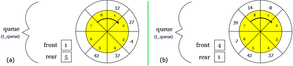
For these two examples, we set Nbmax to 8. Except for the passage of 8 to 1, the values ​​of Head and Tail are increased by 1. This overshoot is simply managed, just using a modulo Nbmax, the value 8 in this case.

Pointer implementation of queues

As for stacks, any list implementation is legal for queues. We can keep two pointers, one to the first element and one to the last one. These pointers are useful for executing enqueue and dequeue operations.

Exaple of algorithmics declaration:

Types

   t_element = ...                   /* element type definition */
   t_prec = $\uparrow$t_rec                   /* t_prec pointer type definition */
   t_rec = record                    /* t_queue type definition */
      t_element elt
      t_prec    next
   end record t_rec

   t_queue = record                   /* queue type definition */
      t_prec front,rear
   end record t_queue

Variables

   t_queue queue

It could correspond to the following structure (a):

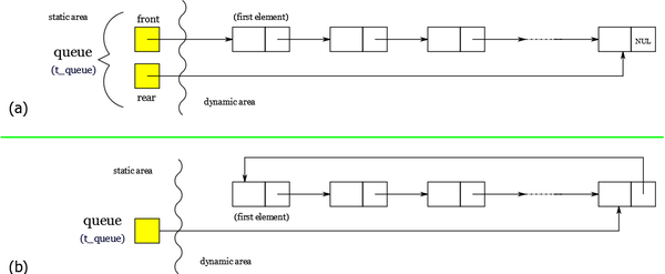
Note that in the case of a circular implementation (b), the front pointer is useless. Just follow the next link from the last element to determine the first element.

---

(Christophe "krisboul" Boullay)