Epita: Algo: Course Info-Spe: graphs
Contents |
General information
There are two kinds of graphs, undirected graphs, for which the connections are symmetric are called edges (figure 1) and directed graphs for which connections are not symmetric and are called directed edges (figure2).
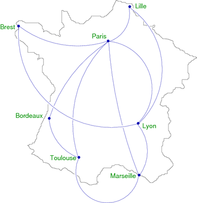
In the following (figure 1) example, the vertices are cities and the relations between these vertices symbolize the existence of an air link. We accept the principle that if there is a flight to go, there is a return flight. The graph is undirected and if two vertices are connected, then we say that there is an edge between these two vertices. For example, there is an edge {Lyon, Strasbourg}. Questions that can be put in this case are: Can we go from Marseille to Brest? (Frankly, if you're in Marseille, who would to go to Brest). Anyway... And in this case, what is the path that requires the least amount of stops?
|
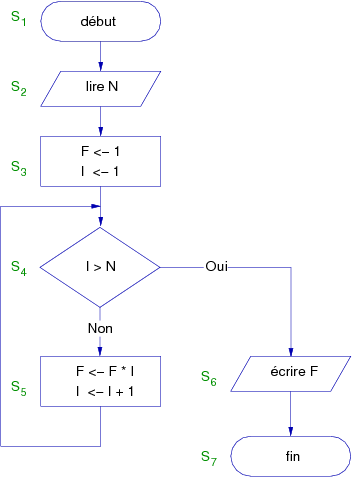
For the following example (figure 2), we have the representation of a flow chart, which calculates the value of the factorial of n. In this case, vertices are blocks of instructions, and the relations symbolize the passage from one block to another but not only. Indeed, they shall also define the direction. For example, you can go from the vertex S2 to the vertex S3, but not vice versa. We say in this case that the graph is directed and the existence of a connection between two vertices is called directed edge or arc. For example, there is an arc ( ).
).
|
Definitions and terminologies
The directed graphs
The multidigraphs
The multidigraphs are the most common form of the directed graphs (digraphs). A multidigraph is an ordered pair < S, A >, with:
- S a finite set of vertices also called nodes in particular cases. The number of vertices of G is call order of G. By convention, we will use the letter N to design the order of G.
- A a multiset (or bag) of ordered pairs of vertices also called directed edges (either arcs or arrows). A multiset is a set in which members are allowed to appear more than once. By convention, we will use the letter M to design the number of arcs of G.
- A multidigraph can be Weighted. It is then defined by a triplet < S, A, C > with C a function, from A to
 , called weight (or cost) function. By convention, we will use Cu to represent the cost, the weight or the value of an arc u.
When the graphs are small (some vertices and relations between these vertices), we can represent it graphically using ordered pairs of endvertices and arrows drawn between the endvertices.
|
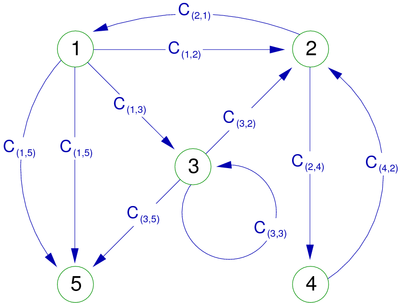
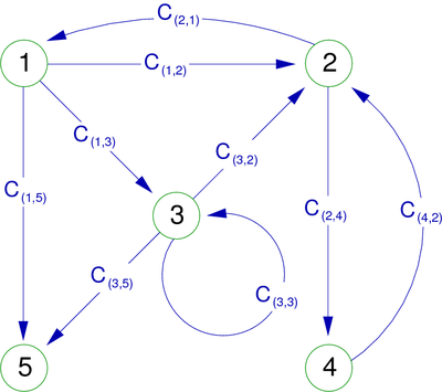
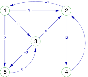
The example of the figure 3 shows a multidigraph of order 5. Indeed, therre are two arcs (1,5) and 5 vertices. This example also has a loop (self-loop), that is to say an arc whose endpoints are the same vertex (in this case the vertex 3).
Remark : A directed graph can be used as an undirected graph when it can be useful. The Paris metro, for example, is by nature oriented (because of some stations) but despite this, for a path search, our interest is to consider it as undirected.
Basic terminology :
- An arc u=(x,y) considered to be directed from x to y is noted u=x
 y, and has two (end-points) such as:
- x is the head of the arc u
- y is the tail of the arc u
- y is the direct successor of x
- x is the direct predecessor of y
- Two arcs of a digraph are considered adjacent if they have at least one common end-point.
- In a digraph, a vertex y is considered adjacent (neighbor) to a vertex x if there exists an arc x y.
Remark: The set of successors of x is noted Γ(x) (big gamma of x), and this of predecessors Γ − 1(x).
- A complete digraph is a directed graph in which every pair of distinct vertices (x,y) is connected by a pair of single edges (one in each direction) x y and y x (the arc inverted).
- In a digraph, if a vertex x is the head of an arc u=x y, we say that the arc u is an outgoing edge (an edge going out of x).
- The number of directed edges going out of a vertex x is called outdegree of x and is noted
 . We note the set of arcs going out of x ω + (x) (omega plus of x) with
 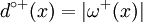 .
.
- In a digraph, if a vertex x is the tail of an arc u=y x, we say that the arc u is an incoming edge (an edge coming into x).
- The number of directed edges coming into a vertex x is called indegree of x and is noted
 . We note the set of arcs coming into x ω − (x) (omega minus of x) with
  .
.
- In a digraph, we call degree of a vertex x the number of arcs connected to it. We note it
 and have
  . The set of arcs incident to x (that x is an endpoint) is noted
  , with obviously
  ..
..
Remarks:
- The loops are counted twice in the degree value
- And isolated vertex is a vertex with degree zero
- When it is ambiguous, we can specify the name of the graph in "sub position", for example:
 , ou
, ou  , etc.
To conclude, in the graph of the figure 3, for the vertex 2 we have:

|
ω − (2) = {(1,2),(3,2),(4,2)} | Γ − 1(2) = {1,3,4} |

|
ω + (2) = {(2,1),(2,4) | Γ(2) = {1,4} |

|
ω(2) = {(1,2),(2,1),(2,4),(3,2),(4,2)} |
The simple digraphs
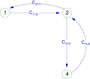
This is the simplest kind of directed graph. For two distinct vertices x and y, there can exist only one directed edge x y. The multi digraph of the figure 3 could become the simple digraph of the figure 4. We can see that one of the two arcs (1,5) has disappeared.
|
In a simple digraph, each arc can be represented, without ambiguity, by a couple (x,y), the multiset (bag) A becomes a set. In the same way, we have | Γ(x) | = | ω + (x) | . (The set of successors of a vertex x is equal to the number of directed edges going out of the vertex x.) This is the same for the previous one, and we also have | Γ − 1(x) | = | ω − (x) | .
We often consider Γ and Γ − 1 as multivalued functions (multifunctions) because they associate with each vertex x of S a set of vertices of S.
Γ is then called successor-function and Γ − 1 predecessor-function. For the graph in figure 4, we would have for each vertex:
| Γ(1) = {2,3,5} |
| Γ(2) = {1,4} |
| Γ(3) = {2,3,5} |
| Γ(4) = {2} |
| Γ(5) = Ø |
In these conditions, we can represent the graph G=< S,A > by G=< S,Γ> where A is replaced by the multifunction Γ (which leads to adjacency lists).
Remarks:
- Thereafter, in this course, we will essentially use simple graph and the word graph will implicitly correspond to simple graph.
- The word graphs refers undirected graphs, the phrase directed graph (digraph) being used for the oriented graphs.
"directed graph" abstract type
The "directed graph" abstract type uses the Vertex type, we give its abstract definition.
types
vertex
uses
integer
operations
ver : integer
axioms
n°(ver(i)) = i
with
integer i
Remark: Thereafter, except in special cases, we will consider vertices as integers.
When we use abstract operations on directed graphs, we assume the following obviousness:
- adding an arc induces the adding of the vertices if they do not belong to the graph.
- the deletion of an arc doesn't induce those of its vertices.
- the deletion of a vertex induces those of all arcs for which it is an endpoint
- adding an existing vertex or an existing arc has no effect.
We will not give the complete algebraic definition of the directed graphs, but only their signature, to which we will add some supplementary functions, to be able to use them in the abstract algorithms we will present, which gives:
types
graph
uses
vertex, integer, boolean
operations
emptygraph :
additional operations
firstsucc : vertex x graph
weighting
weight : vertex x vertex x graph
The undirected graphs
In some cases, such as air travel, the orientation of relations is not important (it is assumed that if we can go, we can return). We are just interested in whether or not two vertices are connected.
The multigraphs
The multidigraphs are the most common form of the undirected graphs. A multidigraph is a pair < S, A >, with :
- S a finite set of vertices also called nodes in particular cases. The number of vertices of G is called order of G. By convention, we will use the letter N to design the order of G.
- A a multiset (or bag) of pairs of vertices also called edges (lines). A multiset is a set in which members are allowed to appear more than once. By convention, we will use the letter M to design the number of arcs of G.
- A multidigraph can be Weighted. It is then defined by a triplet < S, A, C > with C a function, from A to , called weight (or cost) function. By convention, we will use Cu to represent the cost, the weight or the value of an edge u.
When the graphs are small (some vertices and relations between these vertices), we can represent it graphically using ordered pairs of endvertices and arrows drawn between the endvertices.
|
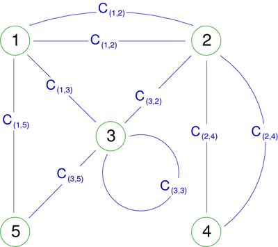
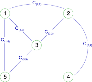
The example of the figure 5 shows a multigraph of order 5. Indeed, there are two edges {1,2}, two edges {2,4} and 5 vertices. This example also has a loop (self-loop), that is to say an arc whose endpoints are the same vertex (in this case the vertex 3).
Basic terminology:
- An edge u={x,y} is noted u=x − y, and has two (end-points) x et y. By analogy with digraphs, we occasionally say that:
- y is the direct successor of x
- x is the direct predecessor of y
and conversely
- Two edges of a graph are considered adjacent if they have at least one common end-point.
- In a graph, two vertices x and y are considered adjacent (neighbor) if there exists an edge x − y.
Remark: As there is no direction, we no longer talk about successors or predecessors, but only about neighbors. The set of neighbors of x is noted Γ(x) (big gamma of x).
- A complete graph is a graph in which every pair of distinct vertices (x,y) is connected by an x − y.
- In a graph, we call degree of a vertex x the number of edges connected to it. We note it and have . The set of edges incident to x (that x is an endpoint) is noted , with obviously ..
Remarks:
- And isolated vertex is a vertex with degree zero
- When it is ambiguous, we can specify the name of the graph in "sub position", for example : , ou , etc.
To conclude, in the graph of the figure 5, for each vertex we have got:

|
ω(1) = {{1,2},{1,2},{1,3},{1,5}} | Γ(1) = {1,3,5} |

|
ω(2) = {{2,1},{2,1},{2,3},{2,4},{2,4}} | Γ(2) = {1,3,4} |

|
ω(3) = {{3,1},{3,2},{3,3},{3,5}} | Γ(3) = {1,2,3,5} |

|
ω(4) = {{4,2},{4,2}} | Γ(4) = {2} |

|
ω(5) = {{5,1},{5,3}} | Γ(5) = {1,3} |
The simple graphs
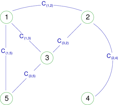
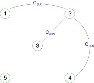
This is the simplest kind of graph. For two distinct vertices x and y, there can exist only one directed edge x y. In this case the interest is not how many edges connect two vertices, but simply whether there is connection between them. Then we keep only an edge between the same two vertices and we ignore the loops. The multigraph in figure 5 could become the simple graph in figure 6. We can see that one of the multiple edges {1,2}, {4,2} and the loop {3,3} has disappeared.
|
Remark: A simple graph is the undirected equivalent to a simple digraph without loop.
We often consider Γ as a multivalued function (multifunction) because it associates with each vertex x of S a set of vertices of S. Γ is then called neighbor-function. For the graph in figure 4, we would have for each vertex:
In these conditions, we can represent the graph G=< S,A > by G=< S,Γ> where A is replaced by the multifunction Γ (which leads to adjacency lists).
Remarks:
- Hereafter, in this course, we will essentially use simple graph and the word graph will implicitly correspond to simple graph.
"undirected graph" abstract type
The "undirected graph" abstract type uses the Vertex type, and we give its abstract definition here.
types
vertex
uses
integer
operations
ver : integer
axioms
n°(ver(i)) = i
with
integer i
Remark: Hereafter, except in special cases, we will consider vertices as integers.
When we use abstract operations on undirected graphs, we assume the following obviousness:
- adding an edge induces the adding of the vertices if they do not belong to the graph.
- the deletion of an edge doesn't induce those of its vertices.
- the deletion of a vertex induces those of all edges for which it is an endpoint
- adding an existing vertex or an existing edge has no effect.
We will not give the complete algebraic definition of the undirected graphs, but only their signature, to which we will add some supplementary functions, to be able to use them in the abstract algorithms we will present, which gives:
types
graph
uses
vertex, integer, boolean
operations
emptygraph :
additional operations
firstneighbor : vertex x graph
weighting
weight : vertex x vertex x graph
The subgraphs and spanning subgraphs
The subgraphs
Let G=< S, A > be a graph (directed or not). The 'subgraph of G generated by S’  S is the graph G’=< S’, A > whose vertex set S’ is a subset of S, and whose adjacency relation is a subset of that of A restricted to S’.
In the other direction, a supergraph of a graph G is a graph of which G is a subgraph.
For a directed graph, that could give :
| graphe G | graphe G' |

|
|
The spanning subgraphs
Let G=< S, A > be a graph (directed or not). The 'spanning subgraph (or factor) of G generated by A’ A is the graph G’=< S, A’ > that has the same vertex set as G. We say G’ spans G.
For an undirected graph, that could give (we will note the vertex 5 isolated) :
| graphe G | graphe G' |
|
|
Paths and connectivities
Definitions
- In a digraph G, we call path an alternating sequence of vertices and directed edges, beginning and ending with a vertex, where each vertex is incident to both the arc that precedes it and the arc that follows it in the sequence, and where the vertices that precede and follow an arc are the end vertices of that arc.
- A path (walk) is closed if its first and last vertices are the same, and open if they are different.
- The length λ of a path (a sequence of (λ + 1) vertices (S0,S1,...,Sλ)), such as
![\forall i \in [0,\lambda-1], S_i\rightarrow S_{i+1}](../images/math/c/4/5/c45b024202484d31669279dd75b7481e.png) is an arc of G), is the number of arcs that it uses.
is an arc of G), is the number of arcs that it uses.
- In a undirected graph G, we call chain an alternating sequence of vertices and edges, beginning and ending with a vertex, where each vertex is incident to both the edge that precedes it and the edge that follows it in the sequence, and where the vertices that precede and follow an edge are the end vertices of that edge.
- The length λ of a chain (a sequence of (λ + 1) vertices (S0,S1,...,Sλ)), such as
![\forall i \in [0,\lambda-1], S_i - S_{i+1}](../images/math/6/c/5/6c502d4a0afadd4de382f7aa5b192aee.png) is an edge of G), is the number of edges that it uses.
is an edge of G), is the number of edges that it uses.
- we consider that the length of a closed path (chain) is equal to 0.
- A path (a chain) in which all vertices are distinct is elementary .
- A closed path (a closed chain) in which all the edges are distinct is a circuit (cycle).
- A directed graph is called strongly connected if there is a path from each vertex in the graph to every other vertex. In particular, this means paths in each direction; a path from x to y and also a path from y to x.
- A graph is called connected if there is a chain between each distinct pair or vertices.
- We call strongly connected components of a directed graph G a maximal strongly connected subgraph. That is to say a strongly connected subgraph which is not strictly included in another strongly connected subgraph.
- We call connected components of a graph G a maximal connected subgraph. That is to say a connected subgraph which is not strictly included in another connected subgraph.
Representations of graphs
There are several ways to represent the graphs. The choice of the representation method depends on many criteria, including the static aspect of the graph. We will present three kinds of representation :
- The adjacency Matrices (for a static set S)
- The adjacency lists (for a static set S)
- The adjacency lists (for an evolving set S).
Adjacency matrix representation
if the set S of n vertices never evolves, it is possible to use a boolean matrix n x n to represent the graph G. We have got the following declaration :
Constants

   NbOfVertices = 4

Types

   t_graph = NbOfVertices x NbOfVertices boolean   /* Definition of the graph matrix representation */

Variables

   t_graph g
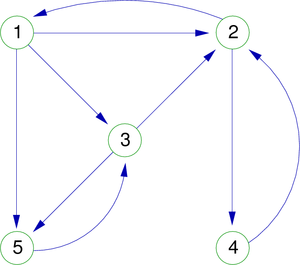
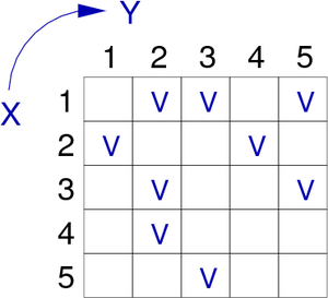
The item g[x,y] is true if a relation exists between the two vertices x and y. In figure 9, we can see an example of a digraph, and its adjacency matrix representation.
remark: To be clear, only the existing arcs are specified V (true).
| Graph G | Adjacency matrix of G |
|
|
Obviously, if the graph is weighted, it is not possible to have only a boolean matrix. In this case, the matrix becomes: either a basic cost matrix (integer, real, etc.) if we do not need the integrality of the definition domain of these types and, that a value can be used to specify the absence of edge, or a user defined cost matrix containing the values and a boolean. We will keep the last proposition which will gives for a graph weighted by elements, the following declaration :
Constants

   NbOfVertices = 4

Types

   t_cost = ...                        /* Cost type definition */
   t_relation = record                 /* Definition of the type t_relation (arc or edge) */
      t_cost  cost
      boolean exist
   end record t_relation

   t_graph = NbOfVertices x NbOfVertices t_relation    /* Definition of the graph matrix representation */

Variables

   t_graph g
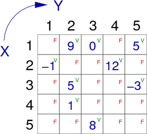
There exists a relation between two vertices i and j if the element G[i,j].exist is True. In figure 10, we can see an example of a weighted digraph, and its adjacency matrix representation in which elements are composed of an integer and a boolean. The latter specifies whether or not the relation (arc or edge) exists between the two concerned vertices.
| Weighted graph G | Adjacency matrix of G |
|
|
Remark: In particular cases, the set of vertices S could evolve slightly. To manage this possibility, it will be necessary to oversize the matrix before starting.
The matrix representation is very covenient to test the existence of an arc. It is easy to add or delete an arc (it is sufficient to switch the field exist to True or to False as the case may be). It is also easy to parse all the successors or the predecessors of a vertex, and to determine its degrees.
The algorithm of the function outdegree determining the out-degree of a vertex x could be :
Algorithm function outdegree : integer Local parameters t_graph g /* g is the graph */ integer x /* x is a vertex of g */ Variables integer d /* d is the temporarly outdegree of x */ integer y /* y is a vertex of g */ Begin d0 /* initializing of d */ for y
Remark: It is sufficient to calculate the in-degree of x to retake this algorithm and to simply test G[y,x].exist.
Unfortunately, a complete traversal of the graph needs a time order of NbOfVertices2 and to stock the graph a memory space of the same order. To solve these problems, we will use another representation called adjacency list.
Adjacency list representation
This representation can have different forms. Actually, it depends on S. If this one is static, we will use an array representation for the vertices, to which a linked list will be attached to specify the successors of each vertex. In the case that S evolves, the array will be replaced by a linked-list.
Static set of vertices
In this case, the declaration of the structure would be the following :
Constants
NbOfVertices = 4
Types
t_cost = ... /* type cost definition */ t_pvertadj =t_vertadj /* Adjacent vertex pointer definition */ t_vertadj = record /* Adjacent vertex definition */ integer numvertadj /* Index number of the adjacent vertex */ t_cost cost t_pvertadj nextvertadj /* pointer on the next adjacent vertex */ end record t_vertadj t_graph = NbOfVertices t_pvertadj /* Graph definition (Array representation of S) */
Variables
t_graph g
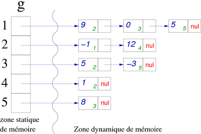
We have got a graph represented by a pointer array on record list corresponding to the adjacent vertices. Each record contains, as an integer, the adjacent vertex number (the index value and this integer gives us the existing edge), the cost if the graph is weighted, and a link (represented by an arrow) to the next adjacent vertex or NUL if there is no other successor (see figure 11).
| Weighted graph G | Adjacency list of G |
|
|
|
Warning: The vertex associated list only contains its successors. This list does not represent a path from the vertex (there is no path (1,2,3), there is no arc (2,3)).
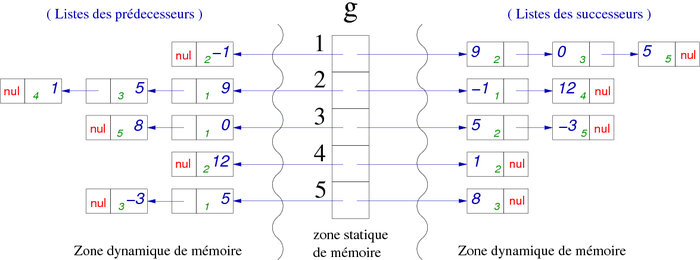
If n is the number of vertices and p the number of arcs, the memory space used for a graph is in order of n + p (multiplied by the size, obviously). For an undirected graph it will be of n + 2p . That is also right for the directed graph for which it will be necessary to have the predecessor list. Indeed, this representation only considers the successors , it is sufficient to have another linked list for the predecessors, as we can see in figure 12 (based on the graph of figure 11).
| Figure 12. Example of adjacency lists (predecessors and successors). |
|
In this case, the structure declaration will be the following :
Constants
NbOfVertices = 4
Types
t_element = ... /* type element definition */ t_cost = ... /* type cost definition */ t_pvertadj =
t_vertadj = record /* Adjacent vertex definition */ integer numvertadj /* Index number of the adjacent vertex */ t_cost cost t_pvertadj nextvertadj /* pointer on the next adjacent vertex */ end record t_vertadj t_graph = NbOfVertices t_pvertex /* Graph definition (Array representation of S) */
Variables
t_graph g
We notice that the array does not contain just one pointer on an adjacent vertex but two (first successor and first predecesor). As it is necessary to have a record for these two fields, we take the opportunity to add a label to the vertex (an element containing all the vertex information). In the case of air link, this label could contain information according to cities, such as latitude, longitude, altitude, etc.
Unfortunately, these representations (matrices or lists) do not allow us to easily modelize a graph with a evolving vertice set.
Dynamic vertices set (evolving)
In the other hand, if the graph has an evolving vertices set, its implementation has to be a linked list to. In this case, the structure declaration will be the following :
Types
t_element = ... /* type element definition */ t_cost = ... /* type cost definition */ t_pvertex =
t_vertadj = record /* Adjacent vertex definition */ t_pvertex vertadj /* pointer on adjacent vertex */ t_cost cost t_pvertadj nextvertadj /* pointer on the next adjacent vertex */ end record t_vertadj t_graph = t_pvertex /* Graph definition (pointer on a vertex) */
Variables
t_graph g
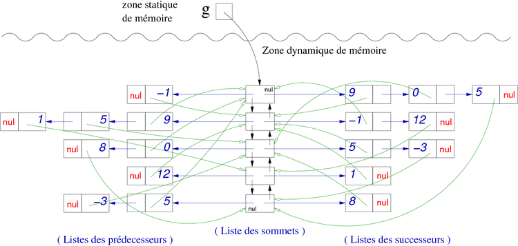
Again, based on the graph in figure 11, that would give the graph in figure 13.
| Figure 13. Example of adjacency lists (predecessors and successors) not static vertices set. |
|
Remarks:
- The vertices list is a double-linked list
- With this kind of representation, it is easy to find an adjacent vertex, to calculate the in-degreee and out-degree of a vertex, and to add or delete a relation between vertices.
- On the contrary, the searching time of an existing arc still stays in time order of n.
Graph traversals (walks)
A traversal is a systematic procedure for exploring a graph by examining all of its vertices and edges. We will consider two efficient traversals of graphs, called depth-first search and Breadth-first search.
Depth-first search
This kind of traversal consists in exploring, starting at a vertex selected as root, as far down as possible along each branch in the graph before backtracking. This traversal is by nature recursive. The major difficulty is not to enter a circuit during the traversal. For that, we will use a "paint" array (vector) that allows us to know if we have already visited a vertex.
Directed graph
Consider a directed graph whose vertices are unpainted. We choose a vertex S, we and it as "visited". We take its first successor (if it exists, obviously…) and then paint it as "visited" and repeat the above computation. When we get to a "dead-end" (no more successor, damn it!), we go back to the previously visited vertex, then repeat the above computation to its second successor, and so on…
Unfortunately if the graph is not strongly connected, it is probable that some vertices were not visited (painted). For this we put an external iterative procedure (dfs_traversal) to verify that the vertices are visited. If it finds one that is not, the traversal procedure (dfs) is called again from the non visited vertex.
The algorithm of depth-first search traversal (recursive version) is:
Algorithm procedure dfs_traversal Constants NbOfVertices = 4 Types t_vectNbool = NbOfVertices boolean Variables t_vectNbool paint /* vector of mark */ t_graph g integer x /* x is a vertex */ Begin for x
Algorithm procedure dfs Local parameters integer x /* x is a vertex */ t_graph g Global parameters t_vectNbool paint /* vector of mark */ Variables integer i,y /* y is a vertex */ Begin paint[x]
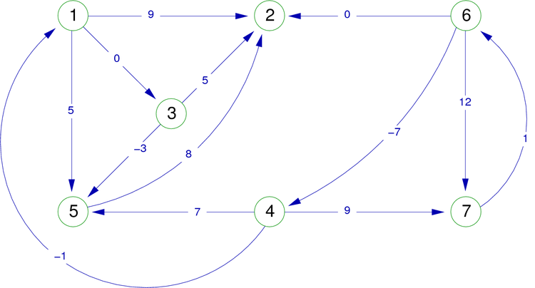
As reference for traversal examples, take the following graph (figure 14).
| Figure 14. Weighted directed graph. |
|
Suppose that the vertices are meeting in increasing order (also for successors), and that the vertex 1 is the first chosen. If using the directed graph in figure 14, we insert in the DFS algorithm a preorder writing instruction of the vertex x (at the first encounter), we will obtain the display of the vertices in the following order:
1, 2, 3, 5, 4, 7, 6
Similarly, if we insert a postorder writing instruction (at the last encounter) of the vertex x, we will obtain the display of the vertices in the following order:
2, 5, 3, 1, 6, 7, 4
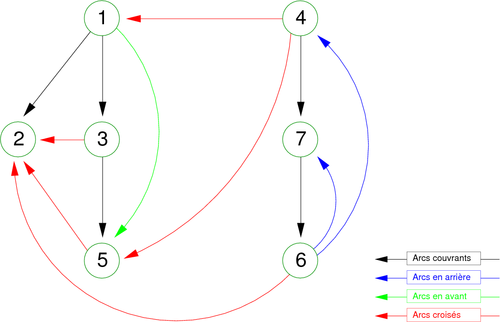
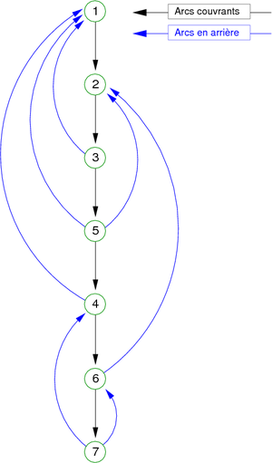
During the depth-first search traversal of a directed graph, if the arcs are drawn when they meet, one obtains for the graph in figure 14 the following graphic representation (figure 15).
| Figure 15. Depth-first search forest associated to the graph in figure 14. |
|
On this representation called Depth-first search forest (spanning forest), associated with the depth-first search walk of the graph g, we can distinguish four kinds of arcs:
- the discovery edges (or tree edges)
- the back edges
- the forward edges
- the cross edges
They correspond to the following definitions:
- Arcs (x,y) such that depth(x) calls depth(y) are called discovery edges. Their set constitutes a spanning forest (depth-first search forest). These are the arcs (1,2), (1,3), (3,5), (4,7) and (7,6) in the given example in Figure 15.
- Arcs (x,y) whose tail is an ancestor of the head in the spanning forest are called back edges. These are the arcs (6,7) and (6,4) in the given example in figure 15.
- Arcs (x,y) whose tail is a descendant of the head in the spanning forest are called forward edges. This is the arc (5,6) in the given example in figure 15.
- Arcs (x,y) for which there is no path between the end-points, in the spanning forest, are called cross edges. These are the arcs (3,2),(5,2),(4,1),(4,5) and (6,2) in the given example in figure 15.
Remarks:
- If by convention, the arcs of the forest are drawn when they are encountered and if the different trees are drawn from left to right, the cross edges will necessarily be directed from right to left.
- As some properties of spanning forests associated with the graph traversals are defined geographically, it is imperative to respect the graphical representation convention mentioned in the previous note.
If during the depth-first traversal of the graph, one assigns to each vertex x a prefix value (pref(x)) which corresponds to its meeting preorder (first met of x), we will obtain the following properties:
- If pref(x)<pref(y) then the arc (x,y) is a discovery edge or a forward edge
- If pref(x)<pref(y) then the arc (x,y) is a back edge or a cross edge
Undirected graph
The used algorithm is the same as for the directed graph. The complexity stays the same insofar as we will consider that a graph with p edges has 2p arcs (remember ?). However, the direction of traversal orients edges and one still speaks of arcs for the associated spanning forest. But we no longer distinguish two types of arcs:
- The discovery edges: Those such as depth(x) = depth(y)+1
- The back edges: Those such as x is a descendant of y in the spanning forest.
Remark:
- If the edge {x,y} has become a discovery edge (during the traversal), we must not to consider it when we build the back edges.
- There is no forward edge since the edges are undirected.
- There is no cross edge since two vertices can not be adjacent without being a descendant of the other one (the relations are symmetrical).
For example, transform the directed graph in figure 14 to the undirected graph in figure 16:
| Figure 16. Weighted undirected graph. |
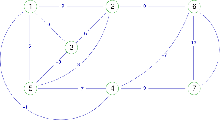
|
Observe the spanning forest obtained in figure 17. As before, suppose that the vertices are meeting in increasing order (also for successors), and that the vertex 1 is the first chosen.
| Figure 17. Spanning forest associated with the graph in figure 16. |
|
Remark: The graph is connected, so the course builds a single tree.
Breadth-first search (level-order)
The traversal begins at a root node and inspects all the children nodes. Then for each of those children nodes in turn, it inspects their children nodes, and so on. In fact, the traversal is done by level (depth in this case), that is to say, at first we traverse all the vertices being at a depth of 1 from the starting vertex, then all vertices being at a depth of 2, and so on...
Remarque : This traversal, also called level-order, is iterative by nature.
In the same way as for the depth-first search traversal, we will "paint" the visited vertices, and if the graph is not connected, it is probable that some vertices were not visited (painted). That is why we put an external iterative procedure (bfs_traversal) to verify that the vertices are visited. If it finds one that is not, the traversal procedure (bfs) is called again from the non visited vertex.
The breadth-first search traversal algorithm (iterative version) uses a queue to memorize the direct successors of each encountered vertex. That allows the next depth to bring the vertices back in their encountered order. That gives the following algorithm:
Algorithm procedure bfs_traversal Constants NbOfVertices = 4 Types t_vectNbool = NbOfVertices boolean Variables t_vectNbool paint /* vector of mark */ t_graph g integer x /* x is a vertex */ Begin for x
Algorithm procdure bfs Local parameters integer x /* x is a vertex */ t_graph g Global parameters t_vectNbool paint /* vector of mark */ Variables integer i,y,z /* y and z are vertices */ queue f /* f stores the descendants of x */ Begin paint[x]
Suppose that the vertices are meeting in increasing order (also for successors), and that the vertex 1 is the first chosen. if using the directed graph in figure 14, we insert in the BFS algorithm a writing instruction of the vertex y at its encounter (y first(f)), we will obtain the display of the vertices in the following order:
1, 2, 3, 5, 4, 7, 6
Remarks:
- In this example, the encountering order of the vertices is the same as for the preorder depth-first traversal. This is absolutely accidental and due to the fact that this example (figure 14) is stupid ;).
- The complexity order is the same as for the depth-first search traversal.
- For this algorithm, the fact that it is iterative makes the inclusion of the main program in the bfs procedure extremely simple. Despite this, it is best to leave things as they are. Indeed, you may want to do the traversal from only one vertex without wanting to traverse the entire graph, which would no longer allow the inclusion.
(Christophe "krisboul" Boullay)