Epita: Algo: Course Info-Spe: Connectivities

Reminders :

• An undirected graph is connected if for all pairs of distinct vertices u et v, there exists a chain (u $\leftrightsquigarrow$ v) connecting these two vertices.
• A directed graph is strongly connected if for all ordered pairs of distinct vertices u et v, there exists a path from u to v (u $\rightsquigarrow$ v).

In this chapter, we are going to present algorithms for determining the connected components of undirected graphs. Then we will use the context of the directed graphs, therefore by extracting of strongly connected components.

Obviously, you can be more demanding and desire that a graph remain connected even after deleting one or more vertices. This property is call the k-connected, k being an integer that gives the maximum number of vertices we can delete while keeping the connectivity property of the graph. We limit ourselves to k = 2.

Connected components

This section will discuss the extraction of connected components of an undirected graph G defined by a pair < S, A >. The analysis of the result is always the same: If we have only one component, the graph is connected, if not, we can determine the vertices of each component and therefore those for which there is a chain ($\leftrightsquigarrow$).

Remark: We assume that the vertices set S is static (fixed) and that the edges set A can be static or evolutive.

Static case

The three ways of determining the connected components of a static undirected graph (S and A fixed) are The depth-first search, The breadth-first search and the calculation of the transitive closure. We already know the first two and we are going to discover the third.

Depth-first search

At the end of the depth-first traversal, we examine the spanning forest associated with it. If there is just one tree the graph is connected, if not there are as many connected components as there are trees and the vertices of each are the nodes that compound the tree.

Breadth-first search

The principle is basically the same as the depht-first traversal, only the encoutering order of the vertices varies (level order).

Transitive closure

Calculating the transitive closure of a graph is used to determine whether the graph is connected.

Definition: We call transitive closure of a graph G defined by the couple < S, A >, the graph G* defined by the couple < S, A* > such that for all pairs of vertices x, y $\in$ S, there exists an edge {x,y} in G* if-and-only-if there exists a chain (of at least one edge) from x to y in G.

Notes:

• The transitive closure G* of a connected graph G is a complete graph
• A graph G is connected if its transitive closure G* is a complete graph
• Two vertices x, y are in the same connected component of G if-and-only-if there exists an edge {x,y} in the transitive closure G* of G.

Formal specification

We will carry out the construction of the transitive closure using successive iterations. This means that to test the existence of a chain between two vertices x and y, we will check if there is one that goes through the vertex s₁, then if there is one that goes through the vertices s₁ and s₂, and so on; Finally if there is one that goes through all vertices of the graph.

Note : If the vertices are integers (1, 2, 3, ...) the calculation of the transitive closure is reduced to simple iteration.

We then define operations iterate and transitiveclosure:

operations

   transitiveclosure : graph $\rightarrow$ graph
             iterate : integer x graph $\rightarrow$ graph

axioms

  /* A graph has the same set of vertices as its transitive closure */
   s isavertexof iterate(i,g) = s isavertexof iterate(i-1,g)

  <s,s'> isanedgeof iterate(i,g) =
         <s,s'> isanedgeof iterate(i-1,g) |
         (<s,i> isanedgeof iterate(i-1,g) & <i,s'> isanedgeof iterate(i-1,g))
  <s,s'> isanedgeof transitiveclosure(g) =
         <s,s'> isanedgeof iterate(nbvertices(g),g)

with

   graph   g
   integer i          /* i > 0 */
   vertex  s, s'      /* s and s' vertices of g */

WARSHALL Algorithm

Principle :

As shown by the previous axioms, there is a chain from a vertex s to a vertex s' going through vertices less than or equal to i, if:

• there is a chain from a vertex s to a vertex s' going through vertices less than or equal to i-1,
• there is a chain from a vertex s to a vertex i going through vertices less than or equal to i-1 and if there is a chain from a vertex i to a vertex s' going through vertices less than or equal to i-1.

Let c be the adjacency matrix of G. In accordance with the specification, we can determine the matrix c* of G*. Suppose that c_i[s,s'] shows the existence of a chain from s' to s' going through vertices less than or equal to i, then we have:

 ci[s,s'] = ci-1[s,s'] or (ci-1[s,i] and ci-1[i,s'])

For the following algorithm, the type of data used is as follows:

Constants

   Nbs = ...                            /* Number of vertices of the graph */

Types

   t_matNbsNbsbool = Nbs x Nbs booléen  /* Boolean square matrix of Nbs vertices */

That gives:

Algorithm procedure Warshall
Local parameters
   t_matNbsNbsbool c                    /* Adjacency matrix of the graph g */
Glocal parameters
   t_matNbsNbsbool c2                   /* Adjacency matrix of the graph g* */
Variables
   integer i, s, s2                      /* i, s and s2 are vertices */
Begin
   /* Initialization of C2 */    
   for s $\leftarrow$ 1 to Nbs do 
      for s2 $\leftarrow$ 1 tgo Nbs do
         C2[s,s2] $\leftarrow$ C[s,s2]
      endfor
   endofr

   /* Calculation of C2 (transitiveclosure) */    
   for i $\leftarrow$ 1 to Nbs do
      for s $\leftarrow$ 1 to Nbs do
         for s2 $\leftarrow$ 1 to Nbs do
            C2[s,s2] $\leftarrow$ C2[s,s2] or (C2[s,i] and C2[i,s2])
         endfor
      endfor
   endfor
End Algorithm procedure Warshall

Note: In the algorithm, we use only one matrix C2 to calculate the successive values of C_i. Indeed, C_i[s,s'] is already equal to C_i-1[s,s'] before each new evaluation. The use of the or operator guarantees us the conservation of true values obtained during previous iterations.

Evolutive case

An undirected graph with n vertices can be known by successively giving its edges. The components of the graph can then be obtained by successive regrouping of components of the evolutive graph.

Indeed, the insertion of an edge x − − − y can modify the set of the connected components of a graph by bringing together that of x with that of y if there are distincts.

We then have to be able:

• to say to which connected component belongs a given vertex,
• to know if two vertices belong to the same component,
• to bring trogether two different components.

Note: Identify the connected components of a graph G, it is building the set of equivalence class for the equivalence relation chain, wherex chain y is true if and only if there is a chain between the two vertices x and y.

More generally, we use the functions find and union to build the partition associated with an evolutionary equivalence relation (relation with instances are known gradually).

These two functions are used as follows:

• find associates with any element of the set on which is defined the equivalence relation, a particular element of its equivalence class (the representative of the Class)
• union Joins two distinct equivalence classes in a single one.

Formal specification

A set with an equivalence relation can be regarded as an undirected graph which satisfies certain properties. The elements of the set are then represented by vertices and the equivalence relation by the edge relation.

Note: If this is undirected graphs, the property of symmetry results from axioms.

In fact, we do not know all the equivalence relations, but only progressively some of them.

As we know that this is an equivalence relation, the explicit addition of a single occurrence (that of an edge in the graph G) is associated with the implicit creation of a certain number of other occurrences (other edges of the graph G*).

This is like building the reflexive and transitive closure of the new graph.

Call closure the operation which performs the construction of the reflective and transitive closure of a graph. Its specification uses the function transitiveclosure previously specified.

So for closure, find and union we have the following specifications:

operations

   closure : graph $\rightarrow$ graph
   /* defined anywhere */
      find : vertex x Graph $\rightarrow$ vertex
   /* Defined only on graphs representing equivalence relations */
     union : vertex x vertex x graph $\rightarrow$ graph
   /* Defined only on graphs representing equivalence relations */

preconditions

   find(s,g) is defined iaoi s isavertexof g = true & g = closure(g)
   union(s,s',g) is defined iaoi s isavertexof g = true &
                                s' isavertexof g = true &
                                g = closure(g)

axioms

   (* A graph has the same set of vertices that its closure *)
   s isavertexof closure(g) = s isavertexof g)
   (* Reflexivity *)
   s isavertexof g = true $\Rightarrow$ <s,s> isanedgeof closure(g) = true
   (* Transitivity *)
   s ≠ s' $\Rightarrow$ <s,s'> isanedgeof closure(g) = <s,s'> isanedgeof transitiveclosure(g)
   (* Two elements of the same equivalence class have the same representative *)
   <s,s'> isanedgeof g = true $\Rightarrow$ find(s,g) = find(s',g)
   (* The representative represents itself *)
   find(find(s,g),g) = find(s',g)
   (* when we add an occurency to the relation (edge), *) 
   (* we build its reflexive and transitive closure *)
   union(s,s',g) = closure(addedge <s,s'> to g)

with

   graph  g
   vertex s, s'      (* s et s' vertices of de g *)

Basic Algorithms

Principle :

We will represent the equivalence classes as a disjoint-set forest. Each tree of the forest has as a root the representative of the associated equivalence class it represents. In this case find(x,G) amounts to searching the tree that contains 'x and returning the root of this tree. If the parent of each item is known, it becomes childish (it's true:)). Moreover, to combine two equivalence classes, it is sufficient to attach the root of one asociated tree to the root of the other one. (That's what I said, a 5 year-old child could do it).

Algorithm :

To represent the disjoint-set forest, we will use an array of n integers, called parent, representatives of the direct ancestors of the nodes in the forest. If a node i $\in$ [1,n] has as a parent a node j $\in$ [1,n], we will have parent[i] = j. If a node i $\in$ [1,n] has no parent (a root) and in this case, we have parent[i] = -1.

Remarks:

• This value will serve as a sentinel in the search for the root of a tree. Indeed, the root of a tree is the only node that has no parent.
• If at the beginning, all equivalence classes are reduced to singletons, our array parent will be entirely initialized by -1.

For the following algorithms, the data type used is:

Constants

   Nbv = ...                  /* Number of vertices of the graph */

Types

   t_vectNbvInt = Nbv integer /* Integer array of direct ancestors */

That gives for find:

/* find(x, parent) returns the root of the tree containing x */
Algorithm function find : integer
Local parameters
   integer      x
   t_vectNbvInt parent                  /* Ancestry Vector */
Begin
   while parent[x] > 0 do
      x $\leftarrow$ parent[x]
   endwhile
   return(x)
Fin Algorithme fontion trouver

An for union:

/* union(x, y, parent) attach the root of the tree containing y */
/* to the root of the tree containing x, if they are distincts */
Algorithm procedure union
Local parameters
   integer      x,y
Global parameters
   t_vectNbvInt parent                  /* Ancestry vector */
Variables
   integer rx,ry
Begin
   rx $\leftarrow$ find(x,parent)
   ry $\leftarrow$ find(y,parent)
   if rx <> ry then
      parent[ry] $\leftarrow$ rx
   endif
End Algorithm procedure union

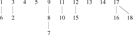
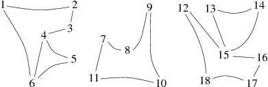
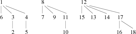
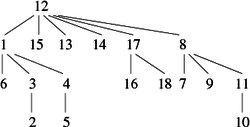
We present an example of graph construction by successive additions of edges. This graph has 18 vertices and its edges are known progressively in the following order:

1 − − − 6, 3 − − − 2, 8 − − − 7, 12 − − − 15, 17 − − − 16, 11 − − − 10, 9 − − − 8, 17 − − − 18, 11 − − − 7, 1 − − − 2, 4 − − − 5, 13 − − − 15, 10 − − − 9, 15 − − − 14, 4 − − − 6, 13 − − − 14, 16 − − − 15, 3 − − − 4, 5 − − − 6, 18 − − − 12

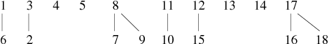
We will cut the construction of the graph in 4 phases. This will allow us to better understand how these algorithms work. We present for each phase (see Tables 1, 2, 3 and 4) , the state of the array parent and the corresponding forest.

Table 1. Phase N°1.

Edges	forest resulting
1 − − − 6, 3 − − − 2, 8 − − − 7, 12 − − − 15, 17 − − − 16, 11 − − − 10, 9 − − − 8, 17 − − − 18
Array parent
vertex 1 2 3 4 5 6 7 8 9 10 11 12 13 14 15 16 17 18 Parent -1 3 -1 -1 -1 1 8 9 -1 11 -1 -1 -1 -1 12 17 -1 17

Table 2. Phase N°2.

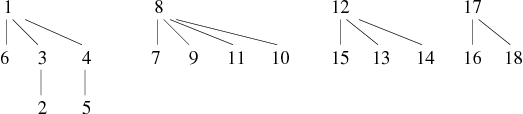
Edges	forest resulting
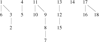
11 − − − 7, 1 − − − 2, 4 − − − 5, 13 − − − 15
Array parent
vertex 1 2 3 4 5 6 7 8 9 10 11 12 13 14 15 16 17 18 Parent -1 3 1 -1 4 1 8 9 11 11 -1 13 -1 -1 12 17 -1 17

Table 3. Phase N°3.

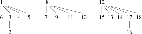
Edges	Forest resulting
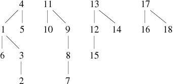
10 − − − 9, 15 − − − 14, 4 − − − 6, 13 − − − 14
Array parent
vertex 1 2 3 4 5 6 7 8 9 10 11 12 13 14 15 16 17 18 Parent 4 3 1 -1 4 1 8 9 11 11 -1 13 -1 13 12 17 -1 17

Table 4. Phase N°4.

Edges	Forest resulting
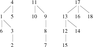
16 − − − 15, 3 − − − 4, 5 − − − 6, 18 − − − 12
Array parent
vertex 1 2 3 4 5 6 7 8 9 10 11 12 13 14 15 16 17 18 Parent 4 3 1 -1 4 1 8 9 11 11 -1 13 17 13 12 17 -1 17

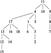
The trees of the final forest are the connected components of the graph. The links are not necessarily those of the graph. In this example, the graph acutally obtained is the one shown in Figure 1 (note that weJ means tree in Klingon, crazy no ?).

Figure 1. weJ Graph.

We can see that the forest obtained has a mamimum depth of 3 for 18 vertices. The form resulting is relatively compact. Unfortunately, it is not always like that. For instance, if we take a graph of n vertices whose n-1 edges are given in the following order:

2 − − − 1, 3 − − − 1, ... , (i-1) − − − 1, i − − − 1, ... , n − − − 1

The forest obtained by successive calls to the procedure union consists of a single tree of depth n-1 and of root n (degenerate tree). In this case, the worst complexity order of find is Θ(n). That is to say that testing the membership of a vertex to a connected component (equivalence class) may take at worst n comparisons.

To avoid this, we propose two improvements that, combined, give something very powerful. The first is:

Union by rank

The idea is as follows: During the addition of an edge x − − − y, rather than attaching systematically the tree containing y to the root of the one that contains x, we will attach the smaller tree (containing fewer elements) to the root of the larger tree.

We call that the union by rank of two trees.

Algorithm:

The difficulty is to find a fast way (even instantaneous) to know the size of a tree at any time. The trick is as follows: For representing the disjoint-set forest, we will also use the array parent. The difference is that if a node i $\in$ [1,n] has no parent, we will have parent[i] = -size with size the number of nodes of the tree whose parent[i] is root (representative).

Remark: Similarly, all equivalence classes are reduced to singletons, so our array parent will be entirely initialized by -1.

That gives for union:

/* union(x, y, parent) attachs the root of the smallest size tree */
/* to the root of the largest size tree if they are distinct*/
Algorithm procedure union
Local parameters
   integer      x,y
Global parameters
   t_vectNbvInt parent                  /* Ancestry Vector */
Variables
   integer rx,ry
Begin
   rx $\leftarrow$ find(x,parent)
   ry $\leftarrow$ find(y,parent)
   if rx <> ry then                     /* The tree of root ry has more elements than this of root rx */
      if parent[rx] > parent[ry] then
         parent[ry] $\leftarrow$) parent[ry]+parent[rx]
         parent[rx] $\leftarrow$ ry
      else
         parent[rx] $\leftarrow$ parent[rx]+parent[ry]
         parent[ry] $\leftarrow$ rx
      endif
   endif
End algorithm procedure union

Remark: If the two trees are of the same size we keep the basic system, which means that the second tree is attached to the root of the first one.

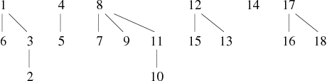
Using the previous example of graph construction by successive additions of edges, keep the cut in 4 phases and observe the results of the application of the new procedure union (see Tables 5, 6,7 et 8).

Table 5. Phase N°1.

Edges	Forest resulting
1 − − − 6, 3 − − − 2, 8 − − − 7, 12 − − − 15, 17 − − − 16, 11 − − − 10, 9 − − − 8, 17 − − − 18
Array parent
vertex 1 2 3 4 5 6 7 8 9 10 11 12 13 14 15 16 17 18 Parent -2 3 -2 -1 -1 1 8 -3 8 11 -2 -2 -1 -1 12 17 -3 17

Table 6. Phase N°2.

Edges	Forest resulting
11 − − − 7, 1 − − − 2, 4 − − − 5, 13 − − − 15
Array parent
vertex 1 2 3 4 5 6 7 8 9 10 11 12 13 14 15 16 17 18 Parent -4 3 1 -2 4 1 8 -5 8 11 8 -3 12 -1 12 17 -3 17

Table 7. Phase N°3.

Edges	Forest resulting
10 − − − 9, 15 − − − 14, 4 − − − 6, 13 − − − 14
Array parent
vertex 1 2 3 4 5 6 7 8 9 10 11 12 13 14 15 16 17 18 Parent -6 3 1 1 4 1 8 -5 8 11 8 -4 12 12 12 17 -3 17

Table 8. Phase N°4.

Edges	Forest resulting
16 − − − 15, 3 − − − 4, 5 − − − 6, 18 − − − 12
Array parent
vertex 1 2 3 4 5 6 7 8 9 10 11 12 13 14 15 16 17 18 Parent -6 3 1 1 4 1 8 -5 8 11 8 -7 12 12 12 17 12 17

The resulting forest now has a maximum depth of 2 which is, due to the small size of the graph, a significant improvement.

That said, we can make the method more efficient by compacting the trees obtained. This is the second improvement and it is called:

Path compression

The idea is as follows: For each call of the function find for a vertex x, we directly hook to the root of the tree that x belongs to, all vertices (including x) lying on the path from x to this root.

For this we will use a new function find, that gives:

/* find(x, parent) returns the root rx of the tree that x currently belongs to */
/* and performs compression between x and rx */
Algorithm function find : integer
Local parameters
   integer      x
Paramètres globaux
   t_vectNbvInt parent             /* Ancestry vector */
   integer rx
Variables
   integer y
Begin
   rx $\leftarrow$ x
   while parent[rx] > 0 do            /* search for rx */
      rx $\leftarrow$ parent[rx]
   endwhile
   while parent[x] <> rx do           /* path compression from x to rx */
      y $\leftarrow$ x
      x $\leftarrow$ parent[x]
      parent[y] $\leftarrow$ rx
   endwhile
   return(rx)
   'endfor
End Algorithm function find

If we combine these two improvements we obtain what we call: The union by rank with path compression.

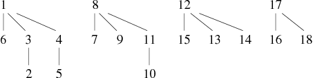
Keeping the previous example of graph construction by successive additions of edges, we can observe the following results: The two first phases are identical to the previous method, the difference comes from the third phase (see Tables 9 and 10).

Table 9. Phase N°3.

Edges	Forest resulting
10 − − − 9, 15 − − − 14, 4 − − − 6, 13 − − − 14
Array parent
vertex 1 2 3 4 5 6 7 8 9 10 11 12 13 14 15 16 17 18 Parent -6 3 1 1 4 1 8 -5 8 8 8 -4 12 12 12 17 -3 17

Table 10. Phase N°4.

Edges	Forest resulting
16 − − − 15, 3 − − − 4, 5 − − − 6, 18 − − − 12
Array parent
vertex 1 2 3 4 5 6 7 8 9 10 11 12 13 14 15 16 17 18 Parent -6 3 1 1 1 1 8 -5 8 8 8 -7 12 12 12 17 12 12

There are some variations as the fact that the vertex 10 is directly attached to 8. Indeed, the addition of the edge 10 − − − 9 does not modify the set of equivalence classes (connected components). Therefore nothing happened with the first version of find. However, the second version (which compresses) takes this opportunity to change the forest. The depth of this latter still has a mamixum of 2, but its average depth has decreased.

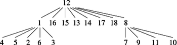
In this example, it is not necessarily very convincing, but if we have reached phase 4, and if we successively add the edges 2 − − − 16 and 10 − − − 18, we will obtain, according to the three methods, the forest in figure 2.

Figure 2. Results of the 3 methods after the addition of the edges 2 − − − 16 et 10 − − − 18.

Basic method	Union by rank	Union by rank & path compression

When we build the equivalence class set of n elements using the union by rank and the path compression methods, finding the equivalence class of an element or checking if two elements belong to the same class, requires at worst a quasi-constant complexity order.

For all sequences of operations, those are union by rank and path compression, if we have m operations find, the time complexity order is at worst Θ(n +m.α (m + n, n)), with α (u, v) a function that grows very slowly, much more slowly than a logarithmic function. It is defined as the inverse of the Ackermann function. In practice, we can consider α (u, v) ≤ 4.

To conclude, once the forest is built we can check at worst if the graph is connected in Θ(n), with n the vertex number (find is called for each vertex).

Note: It's a bit more expensive than the depth-first traversal, but there is no need to store the edges of graph.

Strongly connected Components

We will now consider two methods for determining the strongly connected components (scc) of a directed graph, and thus determining if it is strongly connected. This is the Tarjan algorithm.

• The first method is based on two depth-first traversals with graph inversion,
• The second method uses just one depht-first traversal with the help of a stack.

Kosaraju Algorithm (two depth-first traversals with graph inversion)

Principle: Suppose a directed graph G. Our algorithm stronglyconnectedcomponent will use two traversal procedures: suffdepthtrav and invdepthtrav which respectively realize the following things:

suffdepthtrav: builds a list L of the vertices encountered in the suffix order during the depth-first traversal of the graph' 'G. As usual, we arbitrarily start at the vertex 1 and treat others in ascending order of succession.

invdepthtrav: performs the depth-first traversal of the inverse graph G^-1 and builds the scc vector associating to each vertex its strongly connected component number. To do this, the previously created vertex list L is used in descending order. That is to say that we start by the last element of L (the vertex of greatest suffix value in the depth-first traversal of G) and we go back to the previous unmarked (On returns calls).

Remarks:

• The tree root suffix numbers of the spanning forest G ^-1 are in descending order.
• The subgraphs generated by the vertices of the trees of the obtained spanning forest G ^-1 form the strongly connected components of G.

Algorithm:

For the following algorithm, the data types used are as follows:

Constants

   Nbv = ...                    /* Number of vertices of the graph */

Types

   t_vectNbvInt  = Nbv integer  /* Integer vector */
   t_vectNbvBool = Nbv boolean  /* Boolean vector */

That gives for the main algorithm stronglyconnectedcomponent:

/* After running, cfc[i] will contain the number of the strongly connected component */
/* to which belongs the vertex i */
Algorithm procedure stronglyconnectedcomponent
Local parameters
   graph g
Global parameters
   t_vectNbvInt scc                    /* Vector of strongly connected components */
Variables
   t_vectNbvInt lver                   /* Vertex List */
   t_vectNbvBool mark                  /* Vertex Mark Vector */
   integer i,k
Begin
   /* Initialization */
   for i $\leftarrow$ 1 to Nbv do
      scc[i] $\leftarrow$ 0
      mark[i] $\leftarrow$ False
      lver[i] $\leftarrow$ 0
   endfor
   k $\leftarrow$ 0
   /* K is used as suffix counter */
   /* build the list lver of the vertices of g encountered in the suffix order */ 
   for i $\leftarrow$ 1 to Nbv do
      if not(mark[i]) then
         suffdepthtrav(i,g,mark,lver,k)
      endif
   endfor
   /* Here should take place the reversing of the graph for the next traversal */
   /* Reset Mark to false */
   for i $\leftarrow$ 1 until Nbv do
      mark[i] $\leftarrow$ False
   endfor
   /* K is used as scc detected counter */
   k $\leftarrow$ 0
   for i $\leftarrow$ Nbv downto 1 do
      if not(mark[nth(l,i)]) then
         k $\leftarrow$ k + 1
         invdepthtrav(nth(l,i),g,mark,scc,k)
      endif
   endfor
End algorithm procedure stronglyconnectedcomponent

For the procedure suffdepthtrav :

/* suffdepthtrav(x,g,m,l,k) with x is the root vertex, k is the vertex counter */
/* m the mark vector and l the list of the vertices encountered in prefix order */
Algorithm procedure suffdepthtrav
Local parameters
   integer x
   graph g
Global parameters
   t_vectNbvBool m                     /* Vertex Mark Vector */    
   t_vectNbvInt  l                     /* Vertex list */
   integer       k
Variables
   integer i,y                         /* y is a vertex */
Begin
   m[x] $\leftarrow$ True
   or i $\leftarrow$ 1 to do+(x,g) do
      y $\leftarrow$ nthsucc(i,x,g)
      if not(m[y]) then
         suffdepthtrav(y,g,m,l,k)
      endif
   endfor
   /* suffix vertex processing */
   k $\leftarrow$ k + 1
   l $\leftarrow$ insert(l,k,x)
End algorithm procedure suffdepthtrav

And for the procedure invdepthtrav:

/* invdepthtrav(x,g,m,scc,k) traverses in depth the inverse graph */
/* and fills the table scc with the value k; x is a vertex */
Algorithm procedure invdepthtrav
Local parameters
   integer x
   graph g
Global parameters
   t_vectNbvBool m                     /* Vertex Mark Vector */    
   t_vectNbsEnt  scc                   /* Strongly connected component vector */
   integer        k
Variables
   integer i,y                         /* y is a vertex */
Begin
   m[x] $\leftarrow$ True
   scc[x] $\leftarrow$ k
   /* The trick is not to reverse the graph, but to travel via its predecessors */
   for i $\leftarrow$ 1 to do-(x,g) do
      y $\leftarrow$ nthpred(i,x,g)
      if not(m[y]) then
         invdepthtrav(y,g,m,scc,k)
      endif
   endfor
End algorithm procedure invdepthtrav

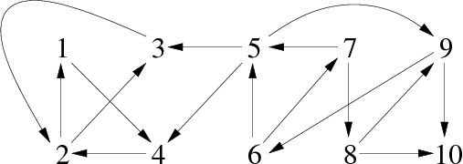
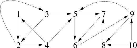
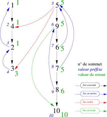
Take for instance the graph G in the figure 3:

Figure 3. Directed graph G.

After running the algorithm suffdephtrav, we obtain the following list lver (represented as a vector to facilitate reading):

Table 11. lver -- List of vertices encountered in suffix order.

Suffix Order (index)	1	2	3	4	5	6	7	8	9	10
Vertices	3	2	4	1	10	8	7	6	9	5

This traversal could be represented graphically as in Figure 4. If we keep only the discovery edges (in black) we see the spanning forest associated to the depth-first traversal of the graph G, which easily allows us to know the suffix order of the vertices of the graph. Again, we start at the vertex 1 and treat others in ascending order of succession.

Figure 4. The spanning forest associated to the depth-first traversal of the graph in figure 3.

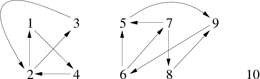
Take now the graph G^-1 (inverse of G) shown in figure 5:

Figure 5. Inverse graph of G (figure 3).

After running the algorithm invdepthtrav, we obtain the following vector scc (table 12) :

Table 12. cfc -- Strongly connected component of each vertex.

Vertices (index)	1	2	3	4	5	6	7	8	9	10
Component Number	3	3	3	3	1	1	1	1	1	2

Remarks:

• The increasing order of the successors is kept, unlike the traversal which has started from the vertex 5 since it has the largest suffix number in lver.

• At the end of the running, the component counter k is equal to 3 (number of strongly connected component of the graph).

Again this traversal could be represented graphically as in Figure 6. If we retain only the discovery arcs, then it becomes easy to identify the trees corresponding to the three strongly connected components of the graph that can be seen in figure 7.

Figure 6. Spanning forest associated to the depth-first traversal of the inverse graph of G (figure 5) using lver in inverse order.

Figure 7. Strongly connected components of the graph in figure 3.

Tarjan algorithm (single traversal and stack)

As we said before, Tarjan algorithm can be optimized to determine the strongly connected components of a graph by performing a single depth-first traversal (It also has its complexity ).

This algorithm exploits the following properties of spanning forests associated with the depth-first traversal of graphs:

• Elementary properties:
  1. Let x and y be two vertices of a same strongly connected component, and let z be a vertex of a path from x to y, so z belongs to the same strongly connected component than x and y.
     
     
  2. Let x and y be two vertices such as it exists a path from x to y. If during a depth-first traversal we mark x while y is not yet marked, y will be in the same tree than x.

• Properties:
  1. Let G=< S, A > be a directed graph and C_i = < S_i, A_i > be a strongly connected component of G with S_i $\subseteq$ S and A_i $\subseteq$ A. Let B_i be the discovery edge set of A_i in the spanning forest associated with the depth-first traversal of G.
     So G_i = < S_i, B_i > is a tree.
     
     Note We call root of the strongly connected component C_i the root r_i of the tree G_i associated with C_i. This is the 1^st vertex of G_i encountered in prefix order.
     
     
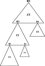
  2. Whatever be i, the vertices of the strongly connected component C_i are the descendants of r_i in the spanning forest associated with the depth-first traversal of G whose are not in the strongly connected components C₁, ..., C_i-1 (see figure 8).

Figure 8. Strongly connected components and their root.

Principle of the algorithm:

The root r _i being considered in suffix order, we obtain the vertices of the strongly connected component C _i taking only the vertices of the tree of root r _i that have not already been taken into account in the previous Components.

We then introduce two funcions that allow us, using the previous properties, to exploit this principle:

• prefix(x): which returns fo each vertex x of the graph G its prefix order number in the depth-first traversal of G.
  
• ret(x): which returns fo each vertex x the prefix order value of a vertex of the strongly connected component of x encountered before it during the depth traversal if it exists or the prefix order value of x itself if not.
  

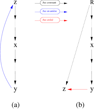
Let z be a vertex. For existing (be a member of the same scc of x and such as prefix(z)<prefix(x)) a such vertex has to be (graphically) placed over and/or at the left of the vertex x. This implies that, starting from x we must follow a path starting with a sequence (possibly empty) of discovery edges continued by a back edge or a cross edge. Graphically: can we find one of the two cases presented in Figure 9?

Figure 9.
Vertex z such as prefix(z) < prefix(x).

• In the case (a), it is clear that, during the depth-first traversal of the spanning forest, the vertex z will be encountered before the vertex x. Therefore Its prefix value will be less than this of the vertex x.

• In the case (b), it is a little more complicated. It must be assumed that prefixe(z) < prefixe(x). From that point:
  • if the two vertices are in the same scc, x is not the root of this component,
  • if not it means that z belongs to another scc (than that of x) encountered before. In this case, the root Rz of the scc of z has a suffix value less than that of the root Rx of the scc of x. Although successor of x in the traversal of the spanning forest, the vertex z has already been assigned to a previous scc.

We then can give a definition of the function return:

return(x) = min { prefix(x), prefix(z), return(y) }

Where the return of x is calculated, at its last encountering (suffix order), on all vertices z and y such as x $\rightarrow$ z is a back edge (figure 9.(a)) or a cross edge (figure 9.(b)) and x $\rightarrow$ y is a discovering edge.

The minimum value returned by ret(x) for each vertex x will be:

• prefix(x) if it does not exist a path from x to z with a vertex z such as prefix(z) < prefix(x).
• prefix(z) if the path from x to z does not contain discovery edges.
• ret(y) if there is at least one discovery edge x $\rightarrow$ y in the path. In this case, the vertex x is able to reach what the vertex y can reach.

Algorithm:

For each vertex x, the evaluation of the return value will be recursively calculated using a depth-first traversal. The vertex is pushed and its return value is initialized with its own prefix value. This value is possibly updated during the encountering of the successors of x (by their prefix value or by their return value.) At the last encountering of the vertex x (suffix order), its return value is compared to its prefix value. In case of equality, we have found a new scc root. Indeed this vertex can not reach any other vertex of the graph which would be encountered before him during the depth-first traversal of this graph. Then just pop all the vertices still in the stack (x included) to get the vertices of this new scc.

The algorithm uses a certain number of arrays to memorize the prefix values, the return values ​​or the scc membership of each vertex of the traversed graph.

For the following algorithm, the data types used are as follows:

Constants

   Nbv = ...                    /* Number of vertices of the graph */

Types

   t_vectNbvInt  = Nbv integer  /* Vector of integers   */

That gives for the main algorithm stronglyconnectedcomponent :

/* After running scc[i] will contain the stongly connected component number */
/* to wich belong the vertx i, and scccpt the number of detected scc */
Algorithm procedure stronglyconnectedcomponent
Local parameters
   graph g
Global parameters
   t_vectNbvInt scc             /* Vector of strongly connected components */
   Integer scccpt               /* Counter of strongly connected components */
Variables
   t_vectNbvInt pref, ret       /* Vectors of prefixe and return values of the vertices */
   integer x, cpt               /* x:vertex, cpt:prefix counter */
   stack p                      /* Stack of vertices */
Begin
   cpt $\leftarrow$ 0
   p $\leftarrow$ emptystack
   /* Initialization */
   for x $\leftarrow$ 1 to Nbv do
      pref[x] $\leftarrow$ 0
   endfor
   /* scc calculation */
   scccpt $\leftarrow$ 0
   for x $\leftarrow$ 1 to Nbv do
      if pref[x]=0 then
         sccdepth(x, g, cpt, scccpt, p, pref, ret, scc)
      endif
   endfor
End Algorithm procedure stonglyconnectedcomponent

For the procedure sccdepth :

/* sccdepth(x, g, cpt, scccpt, p, pref, ret, scc) where x is the root vertex, cpt is the prefix counter of vertices */
/* scccpt the scc counter, p is the stack of vertices, pref the array of prefix value of the vertices (paint vector), */
/* ret the array of return values and scc' the array such as scc[i] gives the scc of i */
Algorithm procedure sccdepth
Local parameters
   integer x
   graph g
Global parameters
   integer cpt,scccpt                   
   stack p   
   t_vectNbvInt  pref, ret, scc
Variables
   integer i, y, min                   /* y is a vertex, min the temporary return value of x */
Begin
   /* Initialization and painting */
   cpt $\leftarrow$ cpt + 1
   pref[x] $\leftarrow$ cpt
   min $\leftarrow$ cpt
   p $\leftarrow$ push(x,p)
   for i $\leftarrow$ 1 to do+(x,g) do
      y $\leftarrow$ nthsucc(i,x,g)
      if pref[y]=0 then   /* y not painted, discovery edge */
         sccdepth(x, g, cpt, scccpt, p, pref, ret, scc)
         if ret[y]<min then   
            min $\leftarrow$ ret[y]
         endif
      else                 /* y already painted, back edge or cross edge */
         if pref[y]<min then   
            min $\leftarrow$ pref[y]
         endif
      endif
   endfor
   ret[x] $\leftarrow$ min
   if ret[x]=pref[x] then       /* news scc whose x is the root */
      cptcfc $\leftarrow$ cptcfc + 1
      while top(p) <> x do
         y $\leftarrow$ top(p)
         scc[y] $\leftarrow$ scccpt
         pref[y] $\leftarrow$ N + 1      
         p $\leftarrow$ pop(p)
      endwhile
      scc[x] $\leftarrow$ scccpt
      pref[x] $\leftarrow$ N + 1
      p $\leftarrow$ pop(p)
   endif
End algorithm procedure sccdepth

After running the algorithm stronglyconnectedcomponent, we obtain the following vector scc (table 13) :

Tableau 13. scc -- Strongly connected component of each vertex.

Vertices (index)	1	2	3	4	5	6	7	8	9	10
N° of component	3	3	3	3	1	1	1	1	1	2

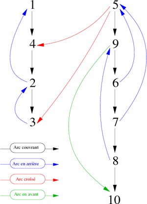
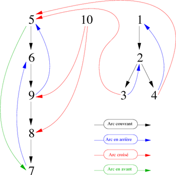
We can visualize the traversal and the way of calculating of the return values of the vertices of the graph using the spanning forest represented in figure 10. There are three strongly connected components determined by their respective root whose prefix and return values are equal (vertices 1, 5 and 10).

Figure 10. Spanning forest associated to the depth-first traversal of the graph G (figure 3).

The strongly connected components are as follows (cf. figure 11):

Figure 11. Strongly connected components of the graph of figure 3.

Biconnected components

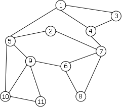
The biconnectivity (2-connectivity) is a property of the connected graphs. This property checks that if one vertex of the graph (any one) is removed, all others remain connected.

Definitions:

• Let G be an undirected connected graph, G is biconnected if it has at least 3 vertices and if for any vertex s of G, the graph G - {s} is still connected.
• Let s be a vertex of G, s is an articulation-point of G (cut-point) if the graph G - {s} is no longer connected.
• Let a be an edge of G, a is an isthmus of G (cut-edge) if the graph G - {a} is no longer connected.

Remark: A biconnected graph has no articulation-points.

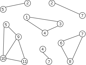
We can see on the example of figure 12.b an undirected connected graph that is not biconnected. It has 4 articulation-points: 2, 4, 5 and 7. Indeed, if you remove one of these vertices, you split the remaining wertices in two distinct groups which are no longer connected to each other.

Figure 12. Connected graphs.

a. 2-connected	b. not 2-connected

2-connexity is used, among other things, to test the vulnerability of networks. In case of conflict, it suffices to destroy the articulation points to separate/weaken an entire communication system.

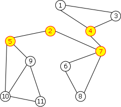
Unfortunately or luckily (it depends;)), not all connected graphs are bi-connected. We are then interested in the biconnected components of the graphs. To define the biconnected components, we introduce the notion of block.

• A block is either an edge, or a biconnected graph.
• We call 2CC (2-connected component) of a graph G all maximal block of G. That is to say a block of G which is not strictly included in another block of G.

Figure 13 shows the set of 2-connected components of the graph of the figure 12b.

Figure 13. 2CC of the graph of figure 12b.

We can note that:

• the C2C form a partition of the set of the edges of the graph,
• C2C are either disjointed or share a point of articulation.

Algorithm:

We propose to perform an algorithm for extracting the articulation-points of an undirected connected graph. It can be modified to determine the 2-connected components of a graph. It performs a single depth-first traversal and examines the properties of the vertices of the spanning forest associated with the depth-first traversal of the graph. This forest is reduced to a tree, because the graph is connected. The graph being undirected, the tree only contains two different types of arcs: discovery and back .

The idea is as follows: when we remove a vertex x of the graph G, we cut the chain which exists between its ascendents and its descendents. The question is: did we lose the connection between these ones?

In other words: Does it exist a chain between the ascendents and the descendents of x in the graph G - {x} ?

If such a chain exists, it will be formed of discovery arcs below x and a back arc going up above x. We will check this possibility using a function higher(x) which will give for each vertex x the prefix order number of the highest vertex of the spanning tree. How ? Following a path, of possibly zero length (if the vertex can not reach an higher vertex than it), composed of discovery arcs possibly followed by a back arc.

The prefix numbering of a vertex x is obtained by the function prefix (x).

The function higher(x) is recursively defined as follows:

higher(x) = min { prefix(x), prefix(z), higher(y) }

Where the higher of x is calculated, at its last encountering (suffix order), on all vertices z and y such as x $\rightarrow$ z is a back edge and x $\rightarrow$ y is a discovering edge.

This definition reminds the return (x) function of the Tarjan algorithm. The difference essentially lies in the fact that there are no cross edges (the graph being undirected).

Principle of the algorithm:

---

(Christophe "krisboul" Boullay)