Epita: Algo: Course: Info-Spe: Hashing methods

A hash function is any algorithm that maps data of variable length to data of a fixed length. The values returned by a hash function are called hash values, hash codes, hash sums, checksums or simply hashes.

hash principle

Let E be a set of names, assume the key is the name itself and that we compute for each item x of the set E, a natural number h(x) called hash value lying between 0 and 8 processed as follows :

• Give to the letter a, b, c, ..., z their own ordinal value, that is to say 1, 2, 3, ..., 26
• Add together the letter's values of the key
• Add to this number the length (the number of letters) of the key
• Compute the remainder of the latter value when it was divided by 9 h(x), to obtain the hash value h(x) $\in$ [0,8]

For the set E = { nathalie, caroline, arnaud, reda, mathieu, jerome, nicolas }, we will obtain the following values :

Table 1. Hashing of E (Values and hash table)

h(nathalie) = (70+8) mod 9 = 6 h(caroline) = (77+8) mod 9 = 4 h(arnaud) = (59+6) mod 9 = 2 h(reda) = (28+4) mod 9 = 5 h(mathieu) = (77+7) mod 9 = 3 h(jerome) = (66+6) mod 9 = 0 h(nicolas) = (73+7) mod 9 = 8 Valeurs de hachage

0 jerome 1 2 arnaud 3 mathieu 4 caroline 5 reda 6 nathalie 7 8 nicolas Associated Hash Table

The table 1 presents the associated hash table to the previous example. We can see that the restriction of h to E is injective (perfect hash function). That is to say that all items x of the set E can be stored in the table and O(1) accesses are required to perform a search in the worst case.

To know if an item x is in E, it is sufficient to compute the table index v = h(x).

 if v = 1 or v = 7 then 
    x is not in E
 else 
    we compare x with the item which is at the index v
    if  x = y then 
       x is in E,
    if' x $\neq$ y then 
       x is not in E

Remark : Obviously, it is necessary to be able to recognize an "empty" box or not.

If you want to add an item x which has the same hash value as another item y already present in the table, h is no longer injective (x $\neq$ y and v = h(x) = h(y)). We call this situation a primary collision between x and y at the slot v.

Later we will see the techniques for resolving the conflict created by collisions. In this case, the fonction no longer gives access to a lone item but to a small group of them.

The set E has been "hashed". This is why the name is hash function.

We use the the hashing methods when we have to store the items of a set belonging to a big universe U. The hash function h maps the universe U into the slots of hash table T[0..m-1] where the size m of the hash table is typically much less than the size of U. The hash function reduces the range of array indices and hence the size of the array. Instead of a size of U, the array can have size m.

For each key x of the set, h(x) (hash value) gives the index of x within the hash table. It allows us to search, insert or delete it. The choice of the hash function is essential, and must be :

• uniform: It should uniformly distribute the set of keys in the hash table,
• easy and fast to compute: The aim is not to weaken the method by a long and tedious calculation,
• Consistent: equal keys must produce the same hash value.

As a result, the design of a hash function is a complex and fastidious issue.

Anyway, and as good as this function might be, we can not avoid collisions. Therefore, we need to know how to manage them. There are, for this purpose, two kinds of methods that we will see later, the methods collision resolution by chaining (indirect methods) and open adressing collision resolution (direct methods).

Hash functions

We now give some principles of construction of a hash function. These are mixable together. We assume for what follows that the keys are represented in memory by a sequence of bits interpreted as integers (natural numbers).

Remark : The advantage of using a sequence of bits is that there is no calculation needed to interprete the value as a natural number.

We must reduce the obtained values to the interval [1,m] or [0,m-1] ( it is often easier to start with 0 ).

For simplicity's sake, we will use characters coded on 5 bits and in increasing progression, that is to say :

A=00001$, B=00010, C=00011, ..., Z=11010

For example :

BUZZ=00010101011101011010

Therefore, the goal is to build the following function h:

$h\ :\ \{0,1\}^{*} \rightarrow [0,m-1]$

set to a bit sequence in a range of m integers.

Extraction method

This method involves extracting a certain number of bits. If p bits are extracted, the interval is reduced to:

[0,2p − 1].

For example, perform the extraction of bits 2, 7, 12 and 17 starting at left and completing with zeros. That gives:

Table 2. Extraction method.

NAT	011100000110100	1000	8
CARO	00011000011001001111	0001	1
REDA	10010001010010000001	0000	0
KRIS	01011100100100110011	1010	10

It's obviously very easy to implement on a computer and in the case of m = 2^p, the obtained word of p bits gives directly an index value in the hash table.

The problem is that the partial use of the key does not give good results. Indeed, a good hash function must use every bit of the key representation. It is well suited in the case where the data is known in advance or when certain bits of the coding are not material.

Compression method

In this method, we use every bit of the key representation that is cut into sub-words of an equal number of bits that are combined with a bit operator. We could use the AND or OR, but they always give values that are lower (ET) or higher (OR) than the original values. For this reason, we prefer using XOR (exclusive OR). For this example, we will use sub-words of 5 bits, which gives:

Table 3. Compression method.

h(NAT)	01110 xor 00001 xor 10100	11011	27
h(CARO)	00011 xor 00001 xor 10010 xor 01111	11111	31
h(REDA)	10010 xor 00101 xor 00100 xor 00001	10010	18
h(KRIS)	01011 xor 10010 xor 01001 xor 10011	00011	3

The problem with this method comes when you "hash" the same way all anagrams of a key, for example:

h(REDA) = 10010 xor 00101 xor 00100 xor 00001 = 10010 = 18
h(READ) = 10010 xor 00101 xor 00001 xor 00100 = 10010 = 18

In this case, it is because the key is cut to the character definition limit (5 bits). That said, we can always introduce an offset that solves the problem. Simply rotate the bits to the right, the first character of 1 bit, the second 2, etc. Which gives:

h(REDA) = 01001 xor 01001 xor 10000 xor 00010 = 10010 = 18
h(READ) = 01001 xor 01001 xor 00100 xor 01000 = 01100 = 12

The example given is reduced to keys of 5 bits, but the interest is to encode the final representation on the size of a memory word.

Division method

This method consists to calculate the remainder of the key value divided by m. Assume m = 23 and we use the previous compression values of the keys, we will obtain :

Table 4. Division method.

NAT = 011100000110100	h(NAT) = 27 mod 23 = 4
CARO = 00011000011001001111	h(CARO) = 31 mod 23 = 8
REDA = 10010001010010000001	h(REDA) = 18 mod 23 = 18
KRIS = 01011100100100110011	h(KRIS) = 3 mod 23 = 3

This is very easy to calculate, but if m is even, all even key (resp. odd) will go in even indices (resp. odd). The same is true if m has small dividers. The solution is to take a prime m. But then again, there may be problems of accumulation.

Multiplication method

let θ be a real number, such that 0 < θ < 1, then we construct the following hash function:

$h(e)=\lfloor\ ((x\ *\ \theta)\ mod\ 1)\ *\ m\ \rfloor$

First, we multiply the key x by θ and extract the fractional part of the result. Then we multiply this value by m (size of the hash table) and take the floor of the result. That will give for θ = 0.5987526325, m=27 and the use of the previous compression values of the keys:

Table 5. Multiplication method.

h(NAT)	$\lfloor(($ 27 $\ *\ 0,5987526325)\ mod\ 1)\ *\ 27\rfloor$	4
h(CARO)	$\lfloor(($ 31 $\ *\ 0,5987526325)\ mod\ 1)\ *\ 27\rfloor$	15
h(REDA)	$\lfloor(($ 18 $\ *\ 0,5987526325)\ mod\ 1)\ *\ 27\rfloor$	20
h(KRIS)	$\lfloor(($ 3 $\ *\ 0,5987526325)\ mod\ 1)\ *\ 27\rfloor$	21

An advantage of the multiplication method is that the value of m is not critical. We typically choose it to be a power of 2 (m = 2^pforsomeintegerp), since we can easily implement the function on most computers. Although this method works with any value of the constant θ, it works better with some value than with others. We should avoid taking θ values too ​​close to 0 or 1 to avoid accumulation at the ends of the hash table. The optimal choice depends on characteristics of the data being hashed, but...

Curiously :D, both values ​​θ that are statistically the most uniform, suggested by Knuth, are :

$\theta\ =\ \frac{\sqrt{5}-1}{2}\ \simeq\ 0.6180339887$

$\theta\ =\ 1\ -\ \frac{\sqrt{5}-1}{2}\ \simeq\ 0.3819660113$

Conclusion : There is no universal hash function. Each function must be adapted to the data it handles and to the application that manages them. We will not forget that it must also be consistent and fast.

Collision resolutions

We assume for what follows that we have a uniform and adequate function hash. Then several possible solutions are available to us to resolve collisions.

By chaining (indirect methods)

In such methods, the elements that collide are chained together. Either outside of the table (hashing with separate chaining) or, in an overflow area (coalesced hashing), if dynamic allocation is not possible (this is rarely seen).

hashing with separate chaining

As we said, with this method, the elements are chained together outside the hash table. Each box in the hash table contains a pointer directed at the head of the list of all stored items that hash to this box.

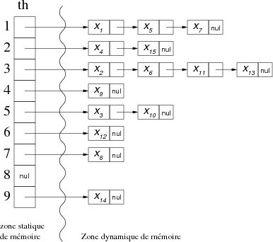
For the following example values:

Table 6. Example of values for separate chaining.

items	X1	X2	X3	X4	X5	X6	X7	X8	X9	X10	X11	X12	X13	X14	X15
hash values	1	3	5	2	1	3	1	7	4	5	3	6	3	9	2

We would have the following hash table th:

Remark: Items in collision could be represented in other forms (trees, etc.), but there is no interest in doing that because if the distribution is uniform and adapted (our premise) to the data set, the number of collisions should not exceed 5, which in search terms (even sequentially: D) is quite "tolerable/acceptable".

Search

Search is simple to implement: it is sufficient to calculate, for the searched element, its hash value, and then to compare each element of the collided elements list (on it) to determine whether it is the one you are looking for.

Insertion

For insertion there are two possibilities :

• Seeking the element to be added, and if it does not exist, insert it at the end of the collision list (we are already at the end of the list after the search). The interest is to keep short lists without redundancy of elements,
• insert at first place in the list of collisions. The advantage is that there is no prior search, thus saving time. The problem is to extend the list of collision (due to the redundancy of elements).

Deletion

As for the insertion, there are two possibilities, the choice depends on the previous choice made for insertion:

• Search for the item to delete and if it exists, delete it,
• Search for all possible instances of the item to be deleted and, optionally, deletion. The main drawback is always having to browse the entire list of collisions.

Coalesced hashing

If dynamic memory allocation is not possible, it is necessary to link the elements together within the hash table. Each slot of the latter has got two fields: an item and a link (usually integer) representing the index of the table where the element in collision is.

The principle is to split the hash table (of size m) in two zones:

• one primary hashing zone of p elements,
• one reserve area of r elements allowing the user to manage the collisions.

The Constraints are, first to have m=p+r greater than or equal to the number of items in the collection to "hash", and second to have a link element, for each index (hash value) within the hash table.

When an item is positionned and its primary hash value reaches an empty box in the main area, it is placed there, otherwise it is placed in the reserve area and the relationship of collision is updated.

Remark : The reserve area is always used in decreasing order of indices.

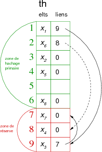
With p=6 and r=3, for the following values of example:

Table 7. Example of values for hashing with reserve area.

éléments	X1	X2	X3	X4	X5	X6	X7	X8
hash values	1	3	1	3	4	2	1	6

we would have the following hash table th:

Remark: In this case, the hash value is no longer calculated on m, but on p.

As we can see, the difficulty lies in the choice of the size of the reserve area. In the previous example, if we wanted to add an element whose primary hash value is 1, 2, 3, 4 or 6, it would collide with another element already present in the table and we would be unable to find a place insofar as the reserve area is already full.

The problem is the following :

• If the reserve area is too small, it is filled too quickly and the use of the table is incomplete,
• If the reserve area is too large, the dispersion effect is lost and extrapolation would give a linked list (which is of no interest).

In this case, a solution is to no longer consider a reserve area, using m at a maximum value and manage primary hash collisions as if there was a reserve area (starting from the maximum index and going up).

The drawback is that this creates collisions that are not due to the coincidence of the primary hash values​​. These are called secondary collisions.

Using this principle and m=17, for the following example values:

Table 8. Example of values for coalesced hashing.

éléments	X1	X2	X3	X4	X5	X6	X7	X8	X9	X10	X11	X12	X13	X14	X15
valeurs de hachage	1	3	5	2	1	3	1	17	4	5	3	14	3	9	2

we would have the following hash table th:

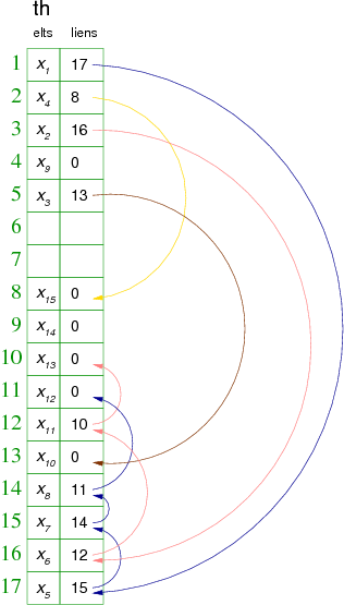
Remark : We directly use the index values for the collision link.

As you can see in the previous example, when inserting x₈ primary hash value 17, we see that its place is already used to manage the collision of x₅ on x₁. Indeed, these two elements have the same primary hash value (1). We solve the problem by putting x₈ at the first free slot in going up (14) and it is linked to its theoretical box (17). In this case, lists of hash values ​​1 and 17 merge, like others thereafter. This phenomenon explains the origin of the name coalesced hashing.

Culture :
Coalesce; come together to form one mass or whole (Oxford Dictionnary)
Origin: mid 16th century: from Latin coalescere "grow together", from co- (from cum "with") + alescere "grow up" (from alere "nourish")

Algorithms

For algorithms that follow, the type of data used is as follows:

Constants

   m = ...                       /* Size of hash table */

Types

   t_element = ...               /* Definition of type of element */
   t_elt = record                /* Definition of type t_elt */
      t_element elt
      integer   lien
   end record t_elt

   t_tabhash = m t_elt           /* Definition of the hash table */

Variables

   t_tabhash th

Searching

Search is simple to implement: it is sufficient to calculate, for the searched element, its hash value, and then to compare each element following the list, using the link, to find the specified element or to find the link to zero.

Remark: we do not waste too much time, since we do not traverse the merged list of collisions from the first element of the first list, but directly from the primary hash value index that we are looking for.

We will write a boolean function that returns "true" if the element exists and "false" otherwise. For this we will use two external functions:

 * h (hashing function)
 * isempty (boolean function returning true if a box is empty)

Function prototypes of h and isempty:

Algorithm function h : integer  /* between 1 and m */
Local parameters
   t_element x

Algorithm function isempty : boolean
Local parameters
   t_tabhash th
   integer   i

Then the search algorithm is:

Algorithm function search_coalescedHashing : boolean
Local parameters
   t_tabhash th
   t_element x
Variables
   integer i
Begin
   i $\leftarrow$ h(x)  /* calculation of the primary hash value */
   if isempty(th,i) then
       return(False)
   endif
   while th[i].elt<>x and th[i].lien<>0 do
       i $\leftarrow$ th[i].lien
   endwhile
   return(th[i].elt=x)
End algorithm function search_coalescedHashing

Insertion

We will use the same functions as for search. The algorithm will also use a variable r (reserve index) which will locate the first slot available (empty) in going up. That gives:

Algorithm function insert_coalescedHashing : boolean
Global parameters
   t_tabhash th
Local parameters
   t_element x
Variables
   integer r, i
Begin
   i $\leftarrow$ h(x)                 /* calculation of the primary hash value */
   r $\leftarrow$ m                    /* initialization of the reserve area slot */
   if isempty(th,i) then     /* insertion of the element */
       th[i].elt $\leftarrow$ x
       th[i].lien $\leftarrow$ 0
       return(True)
   endif
   while th[i].elt<>x and th[i].lien<>0 do
       i $\leftarrow$ th[i].lien
   endwhile
   if th[i].elt=x then      /* element already present */
       return(True)
   endif
   while r>=1 and not(isempty(th,r)) do     /* search of the first empty box in the reserve area*/
       r $\leftarrow$ r-1
   endwhile
   if r>=1 then
       th[i].Lien $\leftarrow$ r       /* update the link with the last item */
       th[r].Elt $\leftarrow$ x        /* in the list of collision on the primary hash value */
       th[r].Lien $\leftarrow$ 0
       return(True)
   endif
   return(False)            /* full table (no way;))*/
End algorithm function insert_coalescedHashing

Remarks :

• the only case of a false return is due to a full table.
• we could memorize r to start systematically from the last slot used for the reserve. In this case, you must keep the search of an 'empty' box. Indeed, it may have had direct insertions of elements (on primary hash value) at the end of table.

Deletion

Except for the separate chaining, it is quite complicated to manage the deletion. Indeed, with the coalesced hashing, deleting an element requires us to eventually shift all those that are linked to it. Its absence can split two collisions lists.

For example, imagine that in the table in figure 8, we remove the element x_x7 located in the the slot of index 15. Then it should shift x_x8 and x_x12. In this case, x_x12 would end up directly in its own primary hash value box that would separate its own collision list of the collision lists of hash value 1 and 17, which would be always linked.

In fact it is preferable in this case not to remove the element, but to create a new process for declaring a box not as empty, but as free. A box may then take three state: empty, free or occupied.

We could then add to the function isempty (previously declared) the functions isfree and isoccupied, but it is more advisable to create just one function which tests the three possible states of a box.

These states are specified by an enumerated type as follows:

Types

   t_state = (empty, free, occupied)             /* Definition of different states of a box */

Therefore a slight modification of the hash table definition is necessary in order to integrate states of each slot, which gives:

Constants

   m = ...                       /* Size of the hash table */

Types

   t_element = ...               /* Definition of the type of elements */
   t_elt = record                /* Definition du type t_elt */
      t_state   state           /* State of the box */
      t_element elt
      integer   link
   end record t_elt

   t_tabhash = m t_elt           /* Definition of the hash table */

Variables

   t_tabhash th

That allows us to specify the function is as follows:

Algorithm function is : boolean
Local parameters
   t_tabhash th
   integer   i
   t_state   state
Begin
   return(th[i].state=state)     /* Comparison of the box state to this one of transmitted parameter */
End algorithm function is

Then the search function becomes :

Algorithm function search_coalescedHashing : integer
Global parameters
   t_tabhash th
Local parameters
   t_element x
Variables
   integer i
Begin
   i $\leftarrow$ h(x)                     /* calculation of the primary hash value */
   while not(is(th,i,empty)) and not(is(th,i,occupied) and th[i].elt=x)  do
      if th[i].link<>0 then
         i $\leftarrow$ th[i].link         /* even if the box is free*/
      else
         break
      endif
   endwhile
   if (is(th,i,occupied) and th[i].elt=x) then
      return(i)
   else
      return(0)
   endif
End algorithm function search_coalescedHashing

Remark: the function has become integer and returns the index value of the searched element if it is found otherwise it is 0.

The delete function consists in searching for the element and, if it exists, changing its box state to "free", it will directly use the search function. It should be noted that this boolean function will return True if the element existed and has been removed and false if not, which gives:

Algorithm function delete_coalescedHashing : boolean
Global parameters
   t_tabhash th
Local parameters
   t_element x
Variables
   integer  i
Begin
   i $\leftarrow$ search_coalescedHashing(th,x)    /* recovery of the box index contening x if it exists, 0 if not*/
   if i>0 then
      th[i].state $\leftarrow$ free
   endif
   return(i>0)
End algorithm function delete_coalescedHashing

In this way, the links are not destroyed and there is no need to rebuild the hash table from the beginning (or at least since the creation of x). To conclude, we need to give the version of the insert fucntion algorithm including the management of boxes freed, which gives:

Algorithm function insert_coalescedHashing : boolean
Global parameters
   t_tabhash th
Local parameters
   t_element x
Variables
   integer r, i, lib
Begin
   i $\leftarrow$ h(x)                                         /* calculation of the primary hash value */
   if is(th,i,vide) then                             /* insertion of the element */
      th[i].elt $\leftarrow$ x
      th[i].link $\leftarrow$ 0
      th[i].state $\leftarrow$ occupied
      return(True)
   endif
   lib $\leftarrow$ 0                                          /* search for the element x */
   while th[i].link<>0 do
      if is(th,i,free) and lib=0 then    
         lib $\leftarrow$ i                                    /* memorizing of the first free box encountered */
      endif   
      if is(th,i,occupied) and th[i].elt=x then
         break
      endif
      i $\leftarrow$ th[i].link                                /* even if the box is free */
   endwhile
   if lib=0 then                                     /* no free box encountered */
      if is(th,i,occupied) and th[i].elt=x then      /* element already présent */
          return(True)
      endif
      r $\leftarrow$ m                                         /* initialization of the reserve area box */
      while r>=1 and not(is(th,r,vide)) do           /* search for the first empty box in the reserve area*/
         r $\leftarrow$ r-1
      endwhile
      if r>=1 then
         th[i].link $\leftarrow$ r                             /* update the link with the last item */
         th[r].elt $\leftarrow$ x                              /* in the list of collision on the primary hash value  */
         th[r].link $\leftarrow$ 0
         th[r].state $\leftarrow$ occupied
         return(True)
      else
         return(False)                             /* full table (no way;))*/
      endif
   else
      th[lib].elt $\leftarrow$ x                               /* list of collision on the primary hash value */
      th[lib].state $\leftarrow$ occupied
      if is(th,i,occupied) andt th[i].elt=x then      /* element already present */
         th[i].state $\leftarrow$ free
      endif   
      return(True)
   endif
End algorithm function insert_coalescedHashing

Remark : The variable lib is used to memorize the first free box encountered during the search for the element. This eventually will allows us to move forward the element x in the list of collision if it already existed. As a reminder, a free box is a box that was occupied by an element that has been deleted in the meantime.

Open Adressing (direct methods)

In such methods, the links no longer exist. The advantage is being able to use their memory space for other elements. The problem is to manage the collisions between elements. The solution is obtained by calculation inside of the table. As for the coalesced hashing, m must be greater or equal to the number of elements to place.

The solution is based on a probe sequence function:

$\begin{matrix}probe &: &E &\rightarrow &\{1, 2, \ldots, m\}^{m} \\  &: &x &\rightarrow &(probe_{1}(x), probe_{2}(x), \ldots, probe_{m}(x)) \end{matrix}$

with 

    $\forall\ i \in \{1,\ldots,m\}\quad probe_{i}(x) \in \{1,\ldots,m\}$

and

    $if\ i \neq j\ then\ probe_{i}(x) \neq probe_{j}(x)$.

Algorithms

For algorithms that follow, the type of data used is as follows:

Constants

   m = ...                       /* Size of the hash table */

Types

   t_element = ...               /* Definition of type of elements */
   t_tabhash = m t_element       /* Definition of hash table */

Variables

   t_tabhash th

Searching

When looking for an element x in the hash table, we successively explore the slots corresponding to the successive trials until we find x or an "empty" box. Indeed, if x existed, it would be placed in the "empty" box.

We will write an integer function that returns the slot index of the element if it exists and 0 if not. For this we will use three external functions:

 * h (hashing function)
 * probe (probe sequence function)
 * isempty (boolean function returning true if a box is empty)

Function prototypes of h, probe and isempty:

Algorithm function h : integer  /* between 1 and m */
Local parameters
   t_element x

Algorithm function probe : integer  /* between 1 and m */
Local parameters
   integer   i                      /* probe number (between 1 and m) */
   t_element x

Algorithm function isempty : boolean
Local parameters
   t_tabhash th
   integer   i

Then the search algorithm is:

Algorithm function search_directHashing : integer
Local parameters
   t_tabhash th
   t_element x
Variables
   integer  i, v                  /* i is the probe number, v is the probe value */
Begin
   i $\leftarrow$ 1            
   while i<=m do
      v $\leftarrow$ probe(i,x)            /* calculation of the ith probe */
      if isempty(th,v) or th[v]=x then
         Break
      endif
      i $\leftarrow$ i+1
   endwhile
   if th[v]=x then
        return(v)
   else
       return(0)
   endif
End algorithm function search_directHashing

Insertion

The procedure is the same as for research. Only when one comes across an "empty" box, do we add the element in this box. The algorithm is globally the same. As it starts with a research phase, we keep the same external functions.

We will therefore write an integer function that returns the index number if the element exists after trying to insert (if it's been created or if it already existed) and 0 if not (full table). The insertion algorithm is:

Algorithm function insert_directHashing : boolean
Global parameters
   t_tabhash th
Local parameters
   t_element x
Variables
   integer  i, v                  /* i is the probe number, v is the probe value */
Begin
   i $\leftarrow$ 1            
   while i<=m do
      v $\leftarrow$ probe(i,x)             /* calculation of the ith probe */
      if isempty(th,v) or th[v]=x then
         Break
      endif
      i $\leftarrow$ i+1
   endwhile
   sif th[v]=x then
        return(v)
   else
      if isempty(th,v) then
         th[v] $\leftarrow$ x
         return(v)
      else
         return(0)
      endif
   endif
End algorithm function insert_directHashing

Remarks :

• It might be wise to check that the table is not full before you start looking. That said, with $m \geqslant n$, it is improbable that happens.
• Using search_directHashing in insert_directHashing is possible, but not very interesting considering the simplicity of the search algorithm. Remember that a function call will take more time than the code "inline".

Deletion

We have shown that deletion generated a problem of data reorganization. We will keep the solution used for the coalesced hashing. We will use the definition of box states as well as the function is which will use the following declarations:

Constants

   m = ...                       /* Size of the hash table */

Types

   t_element = ...               /* Definition of the type of elements */
   t_elt = record                /* Definition du type t_elt */
      t_state   state           /* State of the box */
      t_element elt
   end record t_elt

   t_tabhash = m t_elt           /* Definition of the hash table */

Variables

   t_tabhash th

Then the search function becomes:

Algorithm function search_directHashing : integer
Local parameters
   t_tabhash th
   t_element x
Variables
   integer  i, v                  /* i is the probe number, v is the probe value */
Begin
   i $\leftarrow$ 1            
   while i<=m do
      v $\leftarrow$ probe(i,x)            /* calculation of the ith probe */
      if is(th,v,empty) or (is(th,v,occupied) and th[v].elt=x) then
         Break
      endif
      i $\leftarrow$ i+1
   endwhile
   if is(th,v,occupied) and th[v].elt=x then
      return(v)
   else
      return(0)
   endif
End algorithm function search_directHashing

The deletion procedure only searches for x and sets its state as "free", so:

Algorithm procedure delete_directHashing
Global parameters
   t_tabhash th
Local parameters
   t_element x
Variables
   integer  v                     /* v is the value of the good probe else 0 */
Begin
   v $\leftarrow$ search_directHashing(th,x)
   if v>0 then
       th[v].state $\leftarrow$ free
   endif
End algorithm procedure delete_directHashing

To conclude, it left to give the version of the function insert algorithm including the management of boxes freed, that gives:

Algorithm function insert_directHashing : boolean
Global parameters
   t_tabhash th
Local parameters
   t_element x
Variables
   integer  i, v, lib             /* i is the probe number, v is the probe value, lib the 1st free box */
Begin
   i $\leftarrow$ 1            
   lib $\leftarrow$ 0
   while i<=m do
      v $\leftarrow$ probe(i,x)             /* calculation of the ith probe */
      if is(th,v,empty) then
         Break
      endif
      if is(th,v,occupied) and th[v].elt=x then
         return(v)
      endif
      if is(th,v,free) and lib=0 then
         lib $\leftarrow$ v
      endif
      i $\leftarrow$ i+1
   endwhile
   if is(th,v,empty) then
      if lib=0 then
         th[v].elt $\leftarrow$ x
         th[v].state $\leftarrow$ occupied
         return(v)
      else
         th[lib].elt $\leftarrow$ x
         th[lib].state $\leftarrow$ occupied
         return(lib)
      endif
   else
      return(0)
   endif
End algorithm function insert_directHashing

Remark : As for the coalesced hashing, this algorithm could be modified as follows: as soon as there is a "free"' box or an "empty" box x is inserted. If at the end x is detected and the insertion has been made​​, it is deleted. The interest is to put x as near as possible to its first trial hash value, and thus reduce the time for the next search.

The various techniques of direct hashing are characterized by the choice of the of the probe sequence function. This latter gives a serie of m slots in the hash table. There are at most m! different slots in the table, but most methods use much less. In the linear probing, for example, we see that the sequence of available boxes of an element depends only on the value of primary hash (1st try). This implies that there are only m different sequences in the hash table.

Linear probing

The linear probing works as follows: when there is a collision (when we hash to a table index v that is already occupied with a key different from the search key), then we just check the next entry in the table (by incrementing the index) v+1. If we reach the end (m^th box), we wrap back to the beginning of the table (1^st).

Call Modplus this circular progression and note it $a \oplus b$

Using a uniform hashing function h, the probe sequence will be:

probe1(x) = h(x)

$probe_{2}(x)=h(x) \oplus 1$

...

$probe_{i}(x)=h(x) \oplus i-1$

...

$probe_{m}(x)=h(x) \oplus m-1$

Using this principle and m=11, for the following example of values:

Tableau 9. Example values for the linear probing.

elements	X1	X2	X3	X4	X5	X6	X7	X8	X9
hashing values	10	3	5	11	4	3	1	10	2

We will have the following hash table th:

Remarks :

• Elements which have the same primary hashing value have the same probe sequence.
• Long runs of occupied slots tend to get longer.

An advantage of this technique is there is no need for the conception of a probe sequence function. Indeed, it is sufficient, to replace the first try by a call to the hash function and the other ones by $v \oplus 1$ in the algorithms.

For the search algorithm that would give:

Algorithm function search_linearProbing : integer
Global parameters
   t_tabhash th
Local parameters
   t_element x
Variables
   integer  i, v, lib             /* i is the probe number, v is the probe value, lib is the 1st free box */
Begin
   i $\leftarrow$ 1            
   lib $\leftarrow$ 0
   v $\leftarrow$ h(x)                     /* calculation of the 1st probe */
   while i<=m do
      if is(th,v,empty) or (is(th,v,occupied) and th[v].elt=x) then
         Break
      endif
      if is(th,v,free) and lib=0 then
         lib $\leftarrow$ v
      endif
      i $\leftarrow$ i+1                    
      v $\leftarrow$ v mod m + 1                 /* calculation of the ith probe */
   endwhile
   if lib=0 then
      if i>m then                      /* not found and full table => problem */
         return(0)
      else
         if is(th,v,empty) then        /* not found */
            return(0)
         else                         /* found on v at the ith probe */
            return(v)
         endif
      endif
   else
      if i>m or is(th,v,empty) then    /* not found */
         return(0)
      else
         th[lib].elt $\leftarrow$ x
         th[lib].state $\leftarrow$ occupied
         th[v].state $\leftarrow$ free
         return(lib)
      endif
   endif
End algorithm function search_linearProbing

Remarks :

• The algorithm takes into account the possibility of removing the items and therefore the three possible states of the hash table boxes. This allows two things in the case of searching:
  • differentiate the case not find from the case not found and full table
  • move the founded element to a free slot encountered in its previous trials
• This is of course a simplifiable "rough draft" :)

Double hashing

The linear probing suffers from a problem known as primary clustering due to the buildup of long runs of occupied slots. The probability that a buildup of k elements in a table of size m gets longer at the next insertion is equal to $\frac{k+2}{m}$.

We must therefore try to disperse a few more collided items. We can then imagine the following probe sequence function:

$probe_{i}(x)=h(x) \oplus k(i-1)$

where k is a fixed integer.

To obtain the m hash values during the sequence of m probes, it is necessary that k and m are coprime (mutually prime). In fact, it does not really solve the element buildup problem, but these will occur every k slots. To avoid this, it would been preferable that the increment (k) depend on the element x.

Then we introduce a second hash function d (double hashing) and the probe sequence becomes:

$probe_{i}(x)=h(x) \oplus d(x)(i-1)$

Again each probe sequence must guarantee the m hash values. This requires the same criteria as above, that is to say that m and d(x) have to be coprime regardless of x.

There are two ways to obtain that:

* m is prime and $d \in [1, m-1]$

* m = 2p (it is even) and d(x) has to be odd for all x.
 
  What can be obtained by having d(x) = 2d'(x) + 1, 
  where d'(x) is a fnction whose values are in [0,2p − 1 − 1].

Remark: We will not give the search, insertion and deletion algorithms insofar as the adaptation is very simple (replacement of initializations and of 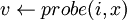$v \leftarrow probe(i,x)$ by $v \leftarrow v \oplus d(x)$ ).

Conclusion on hash methods

• All these methods are well suited for static sets. They are roughly equivalent for a low occupancy rate.

• The coalesced hashing is the most effective method if the memory area reserved for the hashing must be fixed in advance (static data area).

• Linear probing is slower, but this method has the advantage of being extremely simple to implement.

• The double hashing is better than the linear probing, but it requires the computation of two hash functions (and their creation).

• Besides the separate chaining, they do not support deletions well, even with a marking system that significantly increases the search time.

• The most powerful of these is undoubtedly the separate chaining.

---

(Christophe "krisboul" Boullay)