Epita:Algo:Course:Info-Sup: Search Trees

In the basic methods, we saw that we could obtain logarithmic search time using sequential structures with array representation. The ideal would be to get the same performance using dynamic structures. This is not possible with sequential structures, however, it is with tree structures, so ...

The binary search trees (BST)

Any set of n elements whose keys belong to a large universal set that is ordered can be stored and classified within a binary tree of n nodes. In this case, the nodes contain the elements, and parent-child links allow us to manage the order between them.

A BST is a labeled binary tree such that each internal node v stores an element x and :

- Elements stored at nodes in the left subtree of v are less than or equal to x,

- Elements stored at nodes in the right subtree of v are greater than or equal to x,

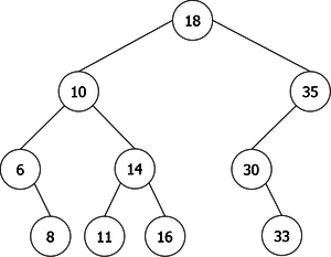
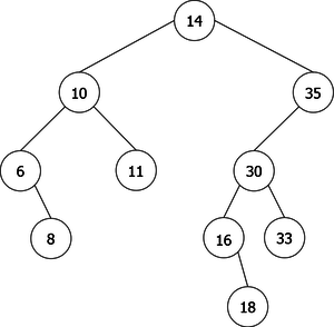
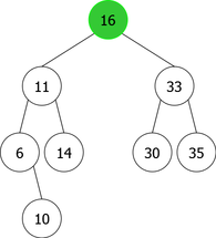
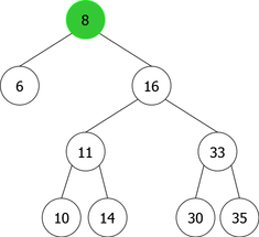
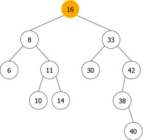
There may be multiple ABRs representing the same data set, as shown in the following example (see Figure 1), the set of integers E = {6,8,10,11,14,16,18,30,33}.

Figure 1. Example of two possible binary search trees of the same set of integers.

Searching in a BST

The search operation of an element x in a BST B defined abstractly by:

operations

   searchBST : element x binarytree $\rightarrow$ boolean

corresponds to the following principle:

- if B is an empty tree, the search terminates unsuccessfully (negative search)
- if x is equal to the element stored in the root node of B the search terminates successfully, (positive search)
- if x is less than the element stored in the root node of B, the search continues in the left subtree of B
- if x is greater than the element stored in the root node of B, the search continues in the right subtree of B

The algorithm corresponding to this principle would be:

Algorithm function searchBST : boolean
Local parameters 
   element  x
   binarytree  B
Begin
   if B = emptytree then   
      return(False)                         /* negative search : fail */
   else   
      if x=content(root(B)) then
         return(True)                       /* positive search : success */
      else
         if x<content(root(B)) then
            return(searchBST(x,l(B)))       /* continuation in the left subtree */
         else
            return(searchBST(x,r(B)))       /* continuation in the right subtree */
         endif
      endif
   endif
End algorithm function searchBST

Insertion in a BST

The operation of adding an element x in a BST B can be done in two ways, at the leaf or at the root of the BST B.

Insertion at the leaf

The adding operation of an element x in a BST B defined abstractly by:

operations

   insertleafBST : element x binarytree $\rightarrow$ binarytree

corresponds to the following principle :

 - finding the position to insert
 - inserting the new element

The first part works on the same principle as the search, the last recursive call ending on an empty tree. It left to create a new node (a new leaf) containing the element x to add. That could give the following algorithm:

Algorithm function insertleafBST : binarytree
Local Parameters 
   element  x
   binarytree  B
Variables
   node  r
Begin
   if B = emptytree then   
      content(r) $\leftarrow$ x
      return(<r,emptytree,emptytree>)  /* a tree with only the new node */
   else   
      if x <= content(root(B)) then
         return(<root(B),insertleafBST(x,l(B)),r(B)>)   /* insertion in the left subtree */
      else
         return(<root(B),l(B),insertleafBST(x,r(B))>)   /* insertion in the right subtree */
      endif
   endif
End algorithm function insertleafBST

Construction of a BST by successive leaf insertions

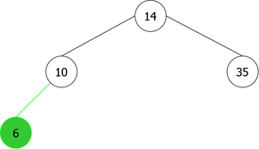
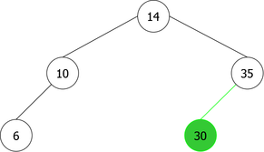
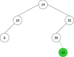
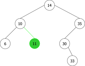
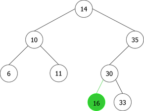
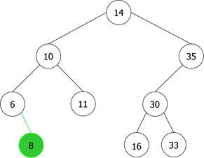
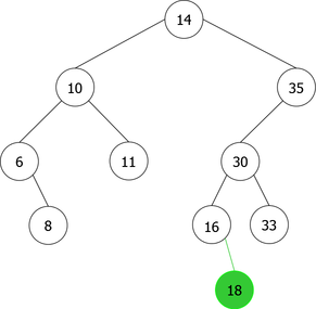
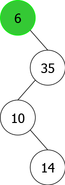
By applying the above algorithm for the following integers : 14, 10, 35, 6, 30, 33, 11, 16, 8, 18 we will obtain the following sequence of the construction of BST :

Figure 2. Construction of a BST by successive leaf insertions of the values 14, 10, 35, 6, 30, 33, 11, 16, 8 et 18.

Root insertion

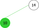
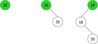
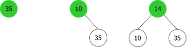
The problem is that we can not just simply add the new element x in a new root node containing it. That would mean positioning it as the left child or right child of the new root. And, it would not certainly respect the order relation, as shown in the sequence of root additions of elements {35, 10, 14} (see Figure 3).

Figure 3. Wrong BST construction by successive insertions of values 35, 10, 14 at root.

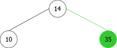
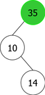
It is clear from this example that after the third root insertion (that of 14), 35 is found in the left sub-tree, which is not possible. Indeed, 35 is greater than 10, but than 14 too. So it should be in the right subtree of the tree of root 14, as shown in Figure 4.

Figure 4. Right BST construction by successive insertions of values 35, 10, 14 at root.

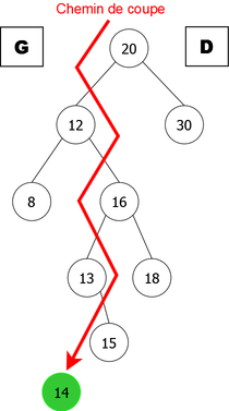
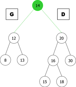
To solve this problem, it should distribute in left subtree (called G) and right subtree (called D) of the new tree created by inserting the new root element x, and the existing elements of B depending on whether they are less than or greater than x.

We will follow the path (called cutting path) from the root of the tree B to the position of the new leaf of B if the insertion is done ​​at the leaf. At each node encountered, we will see if the element is less (resp. greater) than x. If it is less (resp. greater), it will be added to L (resp. R) implicitly with its own left subtree (resp. right) containing elements which are obviously less (resp. greater) than x.

Then it remains to hang L and R to the new root node (containing x), as shown in the example in Figure 5.

Figure 5. Example of insertion at the root of 14 in a BST.

The insertion of an element x at the root of a BST B abstractly defined by :

operations

   insertrootBST : element x binarytree $\rightarrow$ binarytree

will allow us to create the element x, not at a new leaf, but at a new root of the binary tree B. The usefulness of this insertion is, while respecting the order relation, to insert a new element anywhere in a BST (not just at the root).

It corresponds to the following principle:

- Create a new node containing x
- cut the tree B in two trees L and R depending on the cutting path
- hang L and R to the node containing x

Therefore we will need a procedure that cuts a BST B in two subtrees L and R depending on the value of x. This gives the following algorithm:

Algorithm procedure cut
Local parameters
   element  x
Global parameters
   binarytree  B, G, D
Begin
   if B = emptytree then        /* end of recursion and closure of L and R links */
      L $\leftarrow$ emptytree          
      R $\leftarrow$ emptytree
   else
      if x < content(root(B)) then
         R $\leftarrow$ B
         cut(x, l(B), L, l(R))  /* recursion on left subtree and waiting of the left link of R */
      else   
         L $\leftarrow$ B
         cut(x, r(B), r(L), R)  /* recursion on right subtree and waiting of the right link of L */       
      endif
   endif
End algorithm procedure cut

It should be noted that this version of the root insertion algorithm (procedure cut included) does not build trees L and R before hanging them to the new root, but it builds them gradually as it follows the cutting path. In this case, the call of the procedure cut is directly done on the left and right children of the node created as a new root. The calling procedure insertrootBST could be as follows:

Algorithm procedure insertrootBST
Local parameters
   element  x
Global parameters
   binarytree  B
Variables
   binarytree  Aux
Begin
   content(root(Aux)) $\leftarrow$ x
   cut(x, B, l(Aux), r(Aux))   /* call of cut with the left and right children of Aux for L and R */
   B $\leftarrow$ Aux
End algorithm procedure insertrootBST

Construction of a BST by successive root insertions

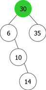
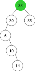
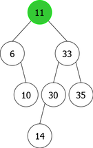
By applying the above algorithm for the following integers : 14, 10, 35, 6, 30, 33, 11, 16, 8, 18 we will obtain the following sequence of the construction of BST :

Figure 6. Construction of a BST by successive root insertions of the values 14, 10, 35, 6, 30, 33, 11, 16, 8 et 18.

Deletion in a BST

The deletion of an element x in a BST B abstractly defined by :

operations

   deleteBST : element x binarytree $\rightarrow$ binarytree

corresponds to the following principle :

- find the element to delete
- delete the element
- eventually reorder the tree

The first part is done with the same principle as the search for an element. After that, it just remains to determine what kind of node we found (the node containing the element x). Indeed, there are three possible cases to consider:

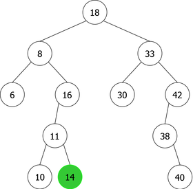
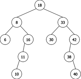
1. The node containing x is a leaf (a node with no children) as in the deletion of 14 (see figure 7(a)). In this case, the node is simply removed and the new tree is that of figure 7(b).
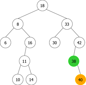
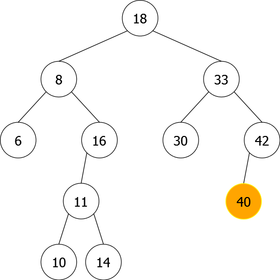
2. The node containing x is a single node (a node with one child), as for the deletion of 38 (right single node) (see figure 8(a)). In this case, the node is simply removed and replaced with its child (the right child in the present example). The tree obtained is that of figure 8(b) where the node 40 replaces its parent, the node 38.
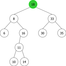
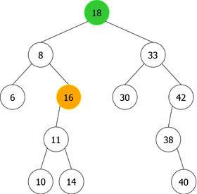
3. The node containing x is a double node (a node with two children), as in the deletion of 18 (root of the tree) (see figure 9(a)). In this case, there exist two possibilities to avoid having to rebuild the tree:
   • Do not delete the node containing x, replace it with its inorder predecessor node (the right-most child of the left subtree), the node 16 in this example.
   • Do not delete the node containing x, replace it with its inorder successor node (the left-most child of the right subtree), the node 30 in this example.

The interest of this method is twofold

• In either case, this node (16 ou 30 in this example) will have one child or none. Delete it according to one of the two simpler cases above.

• the order relation is easily preserved because the biggest of the smaller ones is always smaller than the smallest of the bigger ones, and conversely..
  

In the example of the figure 9, we have chosen to replace the node 18 with its in-order predecessor (the biggest of the smaller ones). The tree obtained is that of the figure 9(b) where the node 16 took the place of the node 18, was deleted and, was itself replaced with its left child (the node 11) as in the second case (single node).

Figure 7. Deletion of the node 14 (leaf).

(a)	(b)

Figure 8. Deletion of the node 38 (right single node).

(a)	(b)

Figure 9. Deletion of the node 18 (double node).

(a)	(b)

Note: These two solutions are equivalent if there is no redundancy of values ​​in the BST.

We will need two additional operations to be able to solve the problem of removing a double node. These two operations are abstractly defined by:

operations

    max : binarytree $\rightarrow$ element
   dmax : binarytree $\rightarrow$ binarytree

and correspond to the following principles:

- max(B) returns the biggest element of the BST B
- dmax(B) returns the BST B amputated of its biggest element

We will merge them in a single operation suppmax, which could give the following algorithm:

Algorithm procedure suppmax
Global parameters
   element     max
   binarytree  B
Begin
   if l(B) = emptytree then       /* no right children, we found the biggest element of the tree */
      max $\leftarrow$ content(root(B))
      B $\leftarrow$ l(B)
   else   
      suppmax(max, r(B))          /* continue on the right */
   endif
End algorithm procedure suppmax

It remains to write the algorithm procedure for deleting an element x in a BST B, which could give the following algorithm:

Algorithm procedure deleteBST 
Local parameters
   element    x
Global parameters
   binarytree B
Variables
   element max
Begin
   if B <> emptytree then   
      if x < content(root(B)) then   
         deleteBST(x, l(B))
      else
         if x > content(root(B)) then   
            deleteBST(x, r(B))
         else       /* x = content(root(B)), x found => deletion. */
            if l(B) = emptytree then    /* B is a right single node or a leaf */
               B $\leftarrow$ r(B)
            else  
               if r(B) = emptytree then /* B is a left single node */
                  B $\leftarrow$ l(B)
               else                     /* B is a double node => call of suppmax */
                  suppmax(max, l(B))
                  content(root(B)) $\leftarrow$ max
               endif
            endif
         endif
      endif
   endif
End algorithm procedure deleteBST

For this algorithm, we have arbitrarily decided to do the search and then manage the deletion when the element is found. We could just as well have done the opposite. This does not change the complexity of this algorithm and in the second case, it would be like the search algorithm that effectively does the "found" before the "try again".

Analysis of the number of comparisons (complexity measures of previous algorithms)

Search, deletion and insertion algorithms work by comparisons of values ​​(x = content(root(B)), x < content(root(B)), x > content(root(B))). The comparison between two elements is the fundamental operation which will allow us to analyze these algorithms and determine their performance. However, the number of comparisons made between two values ​​by these algorithms can be read directly on the BST being worked on, indeed:

• search algorithm:
  • if it ends positively at a node v, the number of comparisons is 2*depth(v)+1
  • if it ends negatively after the node v, the number of comparisons is 2*depth(v)+2

• insertion algorithm:
  • at leaf: the search always ends negatively after a node v. But the number of comparisons is divided by two because one directly asks if x <= content(root(B)). So the number of comparisons is depth(v)+1
  • at the root: the number of comparisons is the same because the algorithm compares the element to insert with those that are in the search path of insertion at leaf (cutting path). The number of comparisons is again depth(v)+1

• deletion algorithm: The number of comparisons is identical to that of the search algorithm. However, if one takes into account the time to search for the replacement element (in case of double point deletion), you must add the complexity of the procedure suppmax.

Conclusion: The analysis (based on the number of value comparisons) of the search for an element, the insertion of an element and the deletion of an element algorithm in a binary search tree is reduced to the study of the depth of nodes in the BST. The average depth of a BST lies between n if the tree is degenerate and $log_2^n$ if it is complete or perfect (see Particular binary trees).

The problem is that these algorithms (insertion and deletion) do not guarantee the balance of the BST and in this case it remains for us to rely on luck or to modify our algorithms so that we will obtain balanced search trees. We will retain the second solution, which, will be dealt with in the next chapter.

Balanced trees

In the previous chapter, we saw that the complexity of the search operation, the insert operation, and the delete operations could be at worst linear. This is because a binary tree is not necessarily balanced, and in the worst case, it can be degenerate. Imagine an insertion at leaf as with successive entries in the list {a, b, c, d, e, f}.

To keep this logarithmic complexity, we need to balance the tree. In this case, it is clear that the reorganization of the tree should be the fastest possible. This will involve a small imbalance of the tree. We will study two classes of balanced trees, the AV.L. (binary tree) and the 2-3-4 trees (general tree). For each of these classes, the time complexities of search algorithm, insertion algorithm, and deletion algorithm will be logarithmic.

Tree rotations

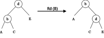
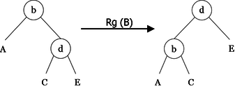
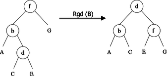
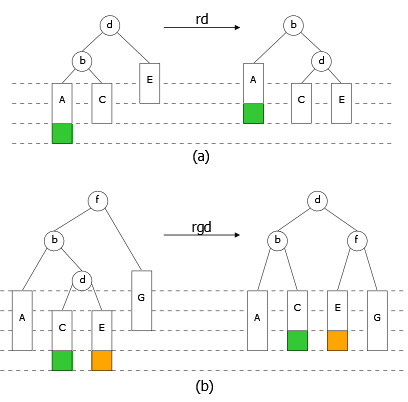
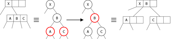
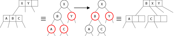
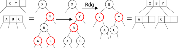
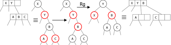
As a first step, we will implement algorithms called rotations for rebalancing. They perform local transformations of the tree that changes the structure without interfering with the order of the elements. They are four in number: two single rotations (left and right), and two double rotations (left-right and right-left). Examples of these rotations are shown in Figures 10, 11, 12 and 13.

Figure 10. Right rotation on the B tree.

Figure 11. left rotation on the B tree.

Figure 12. Left-right rotation on the B tree.

Figure 13. Right-left rotation on the B tree.

Formal specification

These four operations (Lr, Rr, Lrr et Rlr) are abstractly defined by:

operations

   lr  : binarytree $\rightarrow$ binarytree
   rr  : binarytree $\rightarrow$ binarytree
   lrr : binarytree $\rightarrow$ binarytree
   rlr : binarytree $\rightarrow$ binarytree

preconditions

   lr(C) is-defined-iaoi C ≠ emptytree & r(C) ≠ emptytree
   rr(C) is-defined-iaoi C ≠ emptytree & l(C) ≠ emptytree
   lrr(C) is-defined-iaoi C ≠ emptytree & l(C) ≠ emptytree & r(l(C)) ≠ emptytree
   rlr(C) is-defined-iaoi C ≠ emptytree & r(C) ≠ emptytree & l(r(C)) ≠ emptytree

axioms

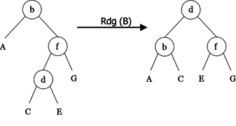
   lr(< b, A, < d, C, E > >) = < d, < b, A, C >, E >
   rr(< d, < b, A, C >, E >)= < b, A, < d, C, E > >
   lrr(< f, < b, A, < d, C, E > >, G >)= < d, < b, A, C >, < f, E, G > >
   rlr(< b, A, < f, < d, C, E >, G > >)= < d, < b, A, C >, < f, E, G > >

with

   binarytree  A, C, E, G
   node        b, d, f

and correspond to the following algorithms:

Left rotation

algorithm procedure Lr
global parameters
   binarytree  B
variables
   binarytree  Aux
begin
   Aux $\leftarrow$ r(B)		/* changes in different links */
   r(B) $\leftarrow$ l(Aux)
   l(Aux) $\leftarrow$ B
   B $\leftarrow$ Aux
end algorithm procedure Lr

Right rotation

algorithm procedure Rr
global parameters
   binarytree  B
variables
   binarytree  Aux
begin
   Aux $\leftarrow$ l(B)		/* changes in different links */
   l(B) $\leftarrow$ r(Aux)
   r(Aux) $\leftarrow$ B
   B $\leftarrow$ Aux
end algorithm procedure Rr

Left-right rotation

algorithm procedure Lrr
global parameters
   binarytree  B
variables
   binarytree  Aux
begin
   Lr(l(B))		/* using simple rotations */
   Rr(B)
end algorithm procedure Lrr

Right-left rotation

algorithm procedure Rlr
global parameters
   binarytree  B
variables
   binarytree  Aux
begin
   Rr(r(B))		/* using simple rotations */
   Lr(B)
end algorithm procedure Rlr

Remarks :

• As can be seen, the double rotations are a combination of two simple rotations. Rotation left-right (right-left) is composed of a rotation left (right) on the left subtree (right subtree) of B followed by a rotation right (left) on B. These two functions are optimizable by replacing two function calls with appropriate assignments. The interest is to avoid both function calls and to reduce the number of assignments from 8 to 6.

• The rotations keep the property of a binary search tree (good deal, right ?). Indeed, we can see that the inorder traversal of B tree, rd(B) tree, rg(B) tree, rgd(B) tree, and rdg(B) tree is the same.

AVL trees

The AVL tree is named after its two Soviet inventors, G. M. Adelson-Velskii and E. M. Landis, who published it in their 1962 paper "An algorithm for the organization of information". It is the first class of height-balanced trees.

Definitions

• We say that a binary tree B = < r, L, R > is Height-balanced if at any node of the tree B the height of the two subtrees (children) of a node differs by at most one. That is to say if height(L) - height(R) $\in$ { -1, 0, +1 }.

• An AVL tree is a Height-balanced (self-balancing) binary search tree.

Formal specification

We need a balance factor operation, abstractly and recursively defined by:

operations

  balancefactor : avl $\rightarrow$ integer

axiomes

  balancefactor(emptytree) = 0
  balancefactor(< r, L, R >) = height(L) - height(R)

with

  avl  B, L, R
  node r

So a binary tree B is Height-balanced if for any subtree C of B we have got: balancefactor(C) $\in$ { -1, 0, 1 }

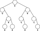
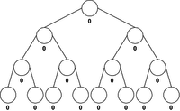
We can see in the figure 14.a an example of Height-balanced trees, and in the figure 14.b an example of a tree that is not.

Figure 14. Examples of height-balanced binary trees (or not).

(a) balanced binary trees	(b) unbalanced binary tree

We will not detail the search algorithm in the AVL. Insofar as they are binary search trees, we can simply keep the search algorithm in the BST. The number of comparisons is always logarithmic.

In contrast, insertion or deletion in an AVL tree can cause an imbalance which can generate a local or complete reorganization of the tree. We will therefore study the insertion algorithm and the deletion algorithm in an AVL tree.

Insertion in an AVL

The principle of creation of an AVL is as follows: We do the insertion of the new element in a leaf. Then we rebalance it if the insertion has unbalanced the tree. In this case, the balance factor we can encounter is at worst ± 2.

If after inserting a node x there is imbalance, it is sufficient to rebalance the tree from a node y located in the path from the root to the leaf x (y may be the root itself ). This node is the last node encountered (closest x) for which the balance factor is ± 2.

Principle of rebalancing

Let B = < r, L, R > an AVL, with no subtrees imbalance ± 2. Assume we insert at a leaf of L an element x, and that the height of the latter increases by 1, and that L remains an AVL (before the insertion in L, its balance factor was 0). In this case, we have got the three following possibilities:

1. if the balance factor of B was 0 before the insertion, it is 1 after. B is always an AVL and its height is increased by 1.
2. if the balance factor of B was -1 before the insertion, it is 0 after. B is always an AVL and its height is not modified.
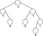
3. if the balance factor of B was 1 before the insertion, it is 2 after. B is no longer balanced, so it's necessary to rebalance it (see. figure 15).

Figure 15. Insertion in an AVL (principle of rebalancing).

As we can see on the Figure 15, the third case has two possibilities :

1. The balance factor of G becomes 1, then the B rebalancing is done using a single right rotation (see figure 15 (a)).

1. The balance factor of G becomes -1, then there is reversal of balance factor between B and G. In this case the the B rebalancing is done using a double right-left rotation (see figure 15 (b)).

In both cases, we recover a balanced binary tree B that is an AVL and whose height is again what it was before inserting the element x (beautiful!).

Remark: Obviously there are the three symmetric cases where the insertion is done on D.

Formal specification

For the insertion in an AVL, we need an operation insertAVL and two operations to manage the imbalance, namely rebalance and balancefactor. The first rebalances the tree, the second lets you know the balance factor of a tree. These operations are defined as follows:

operations

      insertavl  : element x avl $\rightarrow$ avl
       rebalance : avl $\rightarrow$ avl
   balancefactor : avl $\rightarrow$ integer

preconditions

   rebalance(B) is-defined-iaoi balancefactor(B) $\in$ {-2,-1,0,1,2}

axioms

   insertavl( x, emptytree ) = x
   x <= r => insertavl( x, < r, G, D >))= rebalance(< r, insertavl( x, G), D >)
   x > r => insertavl( x, < r, G, D >))= rebalance(< r, G, insertavl( x, D)>)
   balancefactor(B) = -1 => rebalance(B) = B
   balancefactor(B) =  0 => rebalance(B) = B
   balancefactor(B) =  1 => rebalance(B) = B
   balancefactor(B) =  2 & balancefactor(G) =  1 => rebalance(B) = rr(B)
   balancefactor(B) =  2 & balancefactor(G) = -1 => rebalance(B) = lrr(B)
   balancefactor(B) = -2 & balancefactor(D) =  1 => rebalance(B) = rlr(B)
   balancefactor(B) = -2 & balancefactor(D) = -1 => rebalance(B) = lr(B)

with

   avl  B, L, R
   node r
   element x

Remark: It may be noted that there is at most one rebalancing at each insertion.

Algorithm

In terms of implementation, we store in each node the balance factor value of the tree of which it is root. It is therefore necessary to add a field "balfact", taking the values ​​{-2, -1,0,1,2}, in the record type t_node defined for the dynamic representation of binary trees. That gives:

Types

   t_element = ...                /* Definition of type element */
   t_avl = $\uparrow$t_node                /* Definition of type t_avl (pointer-based t_node) */
   t_node = record                /* Definition of type t_node */
      integer   balfact
      t_element elt
      t_avl     lc, lr
   end record t_node

Variables

   t_avl B

Remark: We will stay in an abstract formalism, and for this we use the AVL Data type, which is a derivative of the Binary Tree type that we have added the specific operations to. Some of them, such as, rebalance, will be detailed in the following algorithm.

algorithm procedure insertAVL
global parameters
   avl	B
local parameters
   element x
variables
   avl	Y, A, AA, P, PP
begin
   Y $\leftarrow$ < 0, x, emptytree, emptytree >      /* Creation of node, balfact = 0 */
   if B = emptytree then
      B $\leftarrow$ Y
   else
      A $\leftarrow$ B, AA $\leftarrow$ emptytree              /* AA is the parent of A */
      P $\leftarrow$ B, PP $\leftarrow$ emptytree              /* PP is the parent of P */
      while P <> emptytree do                 /* search of the insertion leaf */
         if balancefactor(P) <> 0 then        /* if a node has a balance factor */
            A $\leftarrow$ P                            /* different from 0, we memorize it */
            AA $\leftarrow$ PP                          /* in A, and its parent in AA  */
         endif
         PP $\leftarrow$ P
         if x <= content(root(P)) then
            P $\leftarrow$ l(P)
         else
            P $\leftarrow$ r(P)
         endif
      endwhile
      if x <= Content(root(PP)) then                    /* Ajout du noeud Y */
         l(PP) $\leftarrow$ Y
      else
         r(PP) $\leftarrow$ Y
      endif
      P $\leftarrow$ A                                           /* imbalance modification */
      while P <> Y do                                  /* on the path from A to Y      */
         if x <= Content(root(P)) then
            balancefactor(P) $\leftarrow$ balancefactor(P) + 1
            P $\leftarrow$ l(P)
         else
            balancefactor(P) $\leftarrow$ balancefactor(P) - 1
            P $\leftarrow$ r(P)
         endif
      endwhile
      case of balancefactor(A) do                                         /* Rebalancing */
         0, 1, -1 : return                                                /* Quit inserting */
                2 : if balancefactor(l(A)) = 1 then                       /* left imbalance */
                       rr(A)                                              /* right rotation */
                       balancefactor(A) $\leftarrow$ 0
                       balancefactor(r(A)) $\leftarrow$ 0
                    else
                       lrr(A)                                             /* left-right rotation */
                       case of balancefactor(A) do
                          -1 : balancefactor(l(A)) $\leftarrow$ 1
                               balancefactor(r(A)) $\leftarrow$ 0
                           1 : balancefactor(l(A)) $\leftarrow$ 0
                               balancefactor(r(A)) $\leftarrow$ -1
                           0 : balancefactor(l(A)) $\leftarrow$ 0                  /* A=Y */
                               balancefactor(r(A)) $\leftarrow$ 0
                       endcase
                       balancefactor(A) $\leftarrow$ 0
                    endif
               -2 : if balancefactor(r(A)) = -1 then                     /* right imbalance */
                       lr(A)                                             /* left rotation */
                       balancefactor(A) $\leftarrow$ 0
                       balancefactor(r(A)) $\leftarrow$ 0
                    else
                       rlr(A)                                            /* right-left rotation */
                       case of balancefactor(A) do
                          -1 : balancefactor(l(A)) $\leftarrow$ 0
                               balancefactor(r(A)) $\leftarrow$ -1
                           1 : balancefactor(l(A)) $\leftarrow$ 1
                               balancefactor(r(A)) $\leftarrow$ 0
                           0 : balancefactor(l(A)) $\leftarrow$ 0                  /* A=Y */
                               balancefactor(r(A)) $\leftarrow$ 0
                       endcase
                       balancefactor(A) $\leftarrow$ 0
                    endif
      endcase
      if AA = emptytree then		/* links updating */
         B $\leftarrow$ A
      else
         if Content(root(A)) <= Content(root(AA)) then
            l(AA) $\leftarrow$ A
         else	
            r(AA) $\leftarrow$ A
         endif
      endif
   endif
end algorithm procedure insertAVL

Deletion in an AVL

The principle of deletion of an element in an AVL is the same as in a binary search tree. That is to say: search for the element to delete, delete it and, if neccessary (in case of double node), replace it with its inorder predecessor node. The problem is that this tree is no longer necessarily H-balanced. We must therefore rebalance it.

After the first phase of deletion, the height of the tree is reduced by 1. If there is imbalance, a rotation is applied. The latter, at its turn, can decrease the height of the tree and generate a new imbalance. And so on up to the root of the tree.

We need to know the path from the root to the deleted node. This involves the use of a stack on an iterative version of the deletion algorithm.

In fact, the principle is simple, if a node x is removed, the height of the tree with root x is examined. If this height has decreased by 1, it may be necessary to use a rotation at the parent of x, and so on.

Formal specification

To delete an element in an AVL, we need the operations rebalance (defined on insertion in an AVL), max and dmax (as defined in the deletion in a BST) and "deleteAVL" that we will define, either:

operations

   deleteAVL : element x avl $\rightarrow$ avl
         max : avl $\rightarrow$ element
        dmax : avl $\rightarrow$ avl

preconditions

   max(B) is-defined-iaoi B <> emptytree
   dmax(B) is-defined-iaoi B <> emptytree

axioms

   deleteAVL( x, emptytree) = emptytree
   x = content(r) => deleteAVL( x, < r, L, emptytree >)) = L
   x = content(r) & R <> emptytree => deleteAVL( x, < r, emptytree, R >)) = R
   x = content(r) & L <> emptytree & R <> emptytree
         => deleteAVL( x, < r, L, R >)) = rebalance(< max(L), dmax(L), R >)
   x < content(r) => deleteAVL( x, < r, L, R >)) = rebalance(< r, deleteAVL( x, L), R >)
   x > content(r) => deleteAVL( x, < r, L, R >)) = rebalance(< r, L, deleteAVL( x, R) >)
   R <> emptytree => max(< r, L, R >) = max(R)
   R <> emptytree => dmax(< r, L, R >)= rebalance(< r, L, dmax(R) >)

with

   avl B, L, R
   node r
   element x

Remark: It may be noted that there could be more than one rebalancing at each deletion.

Algorithm

The deletion algorithm being an exam exercise, it is not included in this handout. I know it would be easier, but hey, nobody provides it, I don't know why I would :)

The 2-3-4 trees

We have seen that to avoid the degeneration of the tree, there was the Height-balanced binary trees. Another possibility is to increase the search axes from a node. In this case, we must use general search trees. So we will use the 2-3-4 trees which are general search trees. Their nodes can contain 1, 2 or 3 elements and all their leaves (external nodes) are at the same depth. This level is the height of the tree that is a logarithmic function of its size (the number of elements it contains). There are functions to rebalance the tree, which can be used after each addition or deletion of an element of the tree. All actions in the 2-3-4 tree are, at worst, logarithmic.

Definitions

A search tree is a general labeled tree whose nodes contain a k-tuple of ordered distinct elements (k = 1, 2, 3, ...). A node containing the items x₁ < x₂ < ... < x_k has k + 1 subtrees, such as:

• all the elements of the first subtree are less than or equal to x₁
• all the elements of the i^th subtree (i = 2, ..., k) are greater than x_{i - 1} and less than or equal to x_i
• all the elements of the (k + 1)^th subtree are greater than x_k

In a search tree, we call k-node a node that contains (k - 1) items.

A 2-3-4 tree is a search tree whose nodes are of three types : 2-node, 3-node or 4-node and all the external nodes (leaves) are at the same depth.

Figure 16. Example of 2-3-4 tree

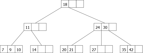
As we can see in figure 16, we have an example of a 2-3-4 tree with 8 nodes containing 13 distinct elements. All items are kept in increasing sorted order and all leaves are at the same depth.

Search in a 2-3-4 tree

The search for an item x in a 2-3-4 tree A works basically as search in a BST. The principle is as follows:

x is compared to the elements x₁, ..., x_i (i = 1, 2 or 3) contained in the root node of A, in this case several possibilities:

• if it exists j $\in$ [1,i] such as x = x_j, then we have found x and the search terminates positively

• if x < x₁, the search of x continues in the 1^st subtree of A

• if x_j < x < x_{j + 1} (j = 1, ..., i - 1), the search of x continues in the (j + 1)^th subtree of A

• if x > x_i, the search of x continues in the last subtree of A

• if the search leads on a leaf that doesn't contain x, then x doesn't exist in A and the search terminates negatively

Remark: The search of an element in a 2-3-4 tree follows a path from the root to a leaf. The depth of the tree being a logarithmic function of the number of elementsof the tree, the worst complexity order of the search algorithm in number of comparisons between elements is always logarithmic.

Insertion in a 2-3-4 tree

We will consider the insertion at bottom. The only problem occurs if the leaf that should receive the new item is already a 4-node (the node is already full). In this case, you will have to create a new node and to rebalance the tree. It is a split function that allows this. Splitting a 4-node can be done:

• either on the way down when searching for the correct place to insert.
• or recursively going up from the bottom.

Insertion with splitting in going up

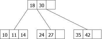
We present an example of successive insertions to the leaves which shows the evolution of the tree. We shall use the following: 30, 11, 35, 18, 27, 42, 14, 10, 24, 7, 21, 9, 20.

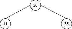
Inserting 30 creates a 2-node which is transformed into 3-node upon the insertion of 11 and after to a 4-node with 35. the evolution is shown in Figure 17.

Figure 17. Insertion of 30, 11 and 35 in a 2-3-4 tree

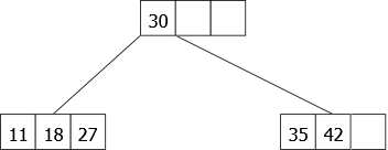
At this stage, inserting an element is impossible, the only leaf is a 4-node. This node could be compared to the binary tree of Figure 18. To insert an item, we will have to split the node by creating two 2-nodes containing the smallest (most-left) and the largest (most-right) element of the node split respectively.

• If the split 4-node is the root of the tree, we create an additional node, so the middle element of the split 4-node becomes the only element of the newly created one and the height of the tree increases by 1.
• If the split 4-node is not a root node, the middle element goes back up to the parent node.

Figure 18. BST equivalent to the 2-3-4 tree of figure 17

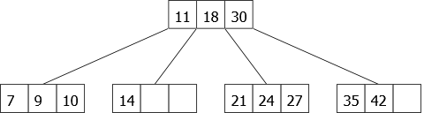
Then we continue on this 2-3-4 tree and we insert 18, 27 and 42, which gives the 2-3-4 tree of figure 19.

Figure 19. Insertion of 18, 27 and 42 in the 2-3-4 tree

The insertion of 14 should be in the first leaf, but it is full. So we have to split it. This is not a root, the middle element (18) goes back up to the parent node and fits naturally (well, it is a way of writing) in its place. Then we will get a new leaf in which the element 14 will be inserted. Then we insert 10 and 24, which gives the tree in Figure 20.

Figure 20. Insertion of 14, 10 and 24 in the 2-3-4 tree

The insertion of 7 splits the first leaf and causes 11 to go up to the root that becomes a 4-node. Then, we insert 21 and 9. That gives the 2-3-4 tree of figure 21.

Figure 21. Insertion of 7, 21 and 9 in the 2-3-4 tree

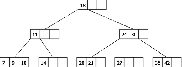
Finally we insert 20. It should be inserted in the third leaf but it's necessary to split. Unfortunately, the ascension of 24 can not be done because its parent node (the root) is also a 4-node. In this case, it will be split too and the height of the tree will increase by 1. That gives the tree of figure 22.

Figure 22. Finally inserting of 20 in a 2-3-4 tree

Insertion with splitting in going down

We will not present the insertion with splitting in going down, but just make a few remarks. Its purpose is to avoid the splitting cascades as generated by inserting the 20 (Figure 22). Indeed, when one traverses the tree seeking for the leaf in which to perform insertion, we systematically split every 4-node encountered. Therefore, there cannot be two consecutive ones. The advantage of this method is that you can write an iterative version of the algorithm without using stack because we do not need to memorize the path from the root to the leaf that is created. The drawback is unnecessarily increasing the height of the tree (by splitting the root) as it could have happened in Figure 21 where we inserted the value 13. This does not require the splitting of the root in the case of an insertion in going up.

Remark: Because both methods operate on a path from the root to the leaf wherein values must be inserted, their complexity order is, in all cases, a logarithmic function of the number of elements of the tree..

Remark 2: In the case of redundancy values​​, two elements of the same value could occur after splits in different nodes. We do not treat these cases. Indeed, the elements of a child node may not be greater than those in the parent node. In this case a change in the definition of 2-3-4 tree and search algorithms and inserting algorithms would be necessary.

Deletion in a 2.3.4. tree

What are the problems caused by removing an element in a 2.3.4. tree?

• As in any tree, deleting an internal node in a 2.3.4. tree causes a problem: it creates orphans! It is simpler to delete an element in a leaf. When the element to delete is in an internal node, we will use the usual method: we replace it either by its immediate predecessor (the largest element of its left subtree), that is to say the lastest element of the right-most leaf; or by its immediate successor (the smallest element of its right subtree), that is to say the first element of the left-most leaf. We will see later what justifies the usage of one or the other possibility.

In fact we always remove an element from a leaf!

• The deletion in a leaf of a 2.3.4. tree causes a problem only if it is a 2-node. Removing the only element would correspond to deleting the leaf, the tree is no longer a tree 2.3.4. (which, we recall, all leaves must be at the same level).

What are the possible solutions?

Just as it is impossible to insert an item in a 4-node, it is impossible to remove an element from a 2-node. The solution will be similar to the one seen for the insertion: the problem of insertion was determined by moving elements in "neighbor" nodes to make room for the new item. For deleting, we have to find additional elements for the inquestion node.

The idea is to move down an element of the parent node. Even if the actual deletion will always be done in a leaf, we will see later that the changes described here will be used for any node types. Let i be the number of the child containing a single element. Two transformations will be used:

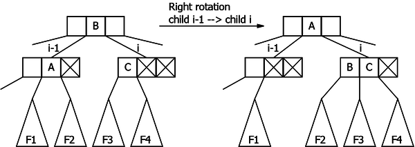
• The rotations

The parent element that moves down is replaced by an element of a sibling of the node. The concerned sibling has to contain at least two elements!

– If the child i-1 (the left sibling) contains at least two elements: the largest one moves up to the parent element (the element i-1) that overlooks the two nodes. The parent element i-1 moves down to the child i to form a 3-node. This is the right rotation (see Figure 22.1). The right child of the "moved up" element becomes the left child of the "moved down" element.

– symmetrically, if the child i+1 (the right sibling) contains at least two elements: the smallest one moves up to the parent element (the element i) that overlooks the two nodes. The parent element i moves down to the child i to form a 3-node. This is the left rotation. The left child of the "moved up" element becomes the right child of the "moved down" element.

Figure 22.1 Right rotation from the child i-1 to the child i

• The fusion (see Figure 22.2)

To use a rotation it is necessary to have one of the two siblings that is not a 2-node. When this is not the case, we will apply the "reverse" transformation of the splitting: the splitting is necessary when there is a maximum occupancy of the nodes, which prevented any insertion. Here we have a minimum occupancy of the nodes: the child i and its two siblings (if they exist) are 2-nodes. The solution is to reduce the number of nodes, by grouping two 2-nodes into one. This is fusion and the principle is as follows:

The child i and the child i+1 (if it exists, otherwise we can do likewise with the child i-1) are grouped into a single node. In the parent node there is one element in the way: the one whose two children have merged. Thus this element moves down in the merged node, where it becomes the middle element. Both elements of the children "take" their children with them.

Figure 22.2 Fusion of the children i and i+1

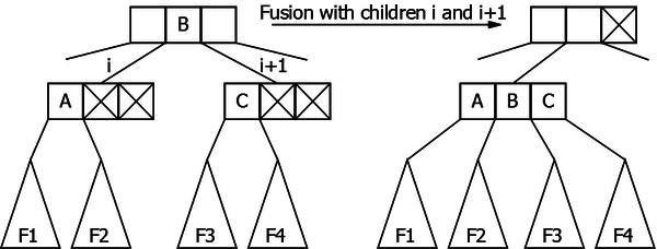
It is important to note that the fusion can not be applied if the parent node is 2-node.

Both transformations presented here require the intervention of the parent node: therefore the transformation of a 2-node will be done before descending on it; the root then becoming a special case.

Principle of deletion in a 2.3.4. tree

Summarize:

• The deletion of an element in a 2.3.4. tree will always be done in a leaf: if the searched element is an internal node, it is sufficient to replace it by its maximum left child, or by its minimum right child (both of which are in a leaf).

• if the node in which we delete is a 2-node, it sufficient either to move an element of one of its siblings (using a rotation) or to perform a fusion with one of its siblings.

Problem!

Doing a rotation is not possible when the sibling nodes are 2-nodes (or the single sibling if it is on an "edge"). Therefore the solution is fusion. For this transformation the parent node can not be a 2-node. What can be done if this is the case?

Once again we are in front of the similar problem of insertion! The first solution consists of transforming the parent node, at its turn, in a node that contains at least two elements. But if its own parent is also a 2-node, we may be faced with the same problem. As the splitting in going up solution, changes can be propagated to the root.

The solution:

We will reapply the precautionary principle: the transformations will be done in going down each time we encounter a 2-node. We are sure to never have two consecutive 2-nodes, and upon arrival on the leaf, the deletion will be done without any problem.

This precautionnay principle implies choosing the replacing element if the element to delete is in an internal node: We will chose the maximum left child if this one is not a 2-node. Otherwise it is the minimum right child that will be used. But if both children are 2-nodes, the solution will be to fusion them (in this case the element to delete will move one level down).

The principle:

Let A be a 2.3.4. tree and x the element to remove. During the traversal of A searching for the key x, it is always necessary to be sure that the node to which we are going down has at least 2 elements (is not a 2-node). The only node authorized to be a 2-node is the root node (we will see thereafter that it is not a problem)! As for insertion, the root must be treated apart in a first procedure (it will also manage the case if the tree is empty or is reduced to a leaf).

The algorithm will be recursive. At each step we are in a non empty tree which has a root node containing at least two elements (except possibly the root of the initial tree).

The first thing to do is to search for the ”place“ of the element in the current node. Let i be this place: either i specifies the searched element number if it is present, or the child number where going down if not. Consider all cases:

• x is not in the current node:

The current node is an internal node:

The current node is a leaf:

if this child i is a 2-node, it is necessary to modify it to increase its number of elements: Either the left sibling, the child i-1 (if it exists) is at least a 3-node, we apply a right rotation. Or the right sibling, the child i+1 (if it exists) is at least a 3-node, we apply a left rotation. Otherwise we perform a fusion, with the right sibling (i+1) if it exists, with the left (i-1) if not. → We start again the deletion of x on the child i (The child i-1 in case of fusionning with the left sibling) which is not a 2-node.

The element does not exist in the tree. → the algorithm stops.

• x is in the current node:

The current node is an internal node:

The current node is a leaf:

The element x must be replaced, if possible, by an element located in a leaf: Either the left child is at least a 3-node and, in this case, we replace the x element by the maximum element of its left subtree → We start again the deletion of its maximum in the left subtree. Or the right child is at least a 3-node and, in this case, we replace the x element by the minimum element of its right subtree → We start again the deletion of its minimum in the right subtree. Otherwise we perform a fusion on the x element → We start again the deletion of x on the resulting child of the fusion.

This node inevitably has two elements → We directly remove the x element.

Implementation of the principle:

Initial tree:

Figure 22.3 Deletion: Initial 2.3.4. tree

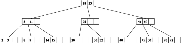
Deletion of the element 32: Before going down on the node {25}, we perform a right rotation (element 11 moves up in the parent node, element 18 moves down in our node. We go down until 32 which we remove.

Figure 22.4 Deletion of the element 32

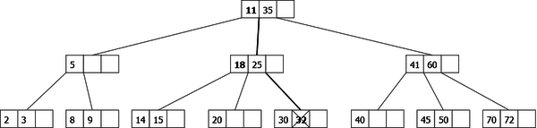
Deletion of the element 25: The left and right children of 25 are 2-nodes, therefore we move down this element fusionning with its two children. 25 is removed in the resulting leaf of the fusion.

Figure 22.5 Deletion of the element 25

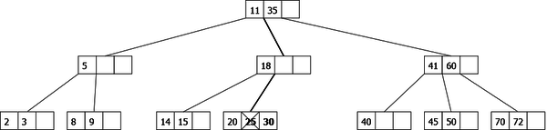
Deletion of the element 35: 35 is in the root node: we replace it by the smallest element of its right child (that is not a 2-node). Then we continue the deletion of this element: 40. The node that contains 40 is a 2-node, we perform a left rotation before going down on it to delete the element.

Figure 22.6 Deletion of the element 35

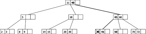
Deletion of the element 5: 5 is in the first child which is a 2-node. There is no possible rotation while its right sibling is also a 2-node. So we start by performing a fusion with the two first siblings, then we go down on the resulting node that contains 5 which is replaced by its maximum left child that we remove.

Figure 22.7 Deletion of the element 5

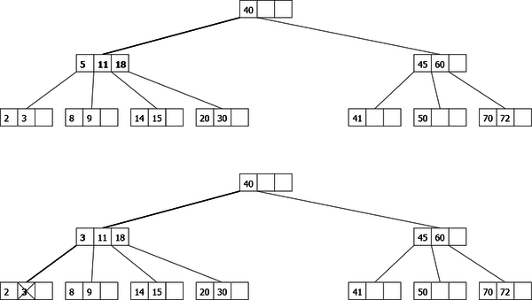
Implementation of 2-3-4 trees

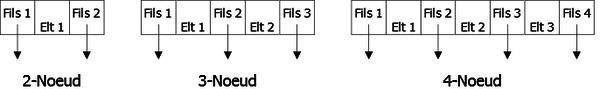
There are different ways to represent the 2-3-4 tree. The first consists in creating, for each kind of node, its own representation as shown in figure 23.

Figure 23. Separate representation of the 2-node, 3-node and 4-node

This minimizes the necessary memory, but makes implementation more complex, since it is necessary to manage each transaction for each kind of node.

Another possibility is the maximal representation. This means that we always take the representation of the 4-node for all kinds of nodes as shown in Figure 24. In this case, if the node is a 2-node, we will only use the first three fields of the structure.

Figure 24. Maximal representation of a 2-3-4 tree

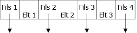
The problem in this case is a waste of memory for every node that is not a 4-node. On the other hand, the removal of an element may require shifting elements and pointers to children. A possibility of simplification is to build a structure containing two tables: one of three elements and four pointers. That would give:

Constants

   MaxElt  = 3                    /* Maximum number of elements */
   MaxFils = MaxElt + 1

Types

   t_element = ...                /* Type definition of elements */
   t_a234    = $\uparrow$t_noeud234       /* Type definition of t_a234 (pointer on t_node234) */
   t_vectElt = MaxElt t_element   /* Element array */
   t_vectFils = MaxFils t_a234    /* Array of pointers on child */
   t_noeud234 = enregistrement
     t_vectElt  elts
     t_vectFils fils
   fin enregistrement t_noeud234

Variables

   t_a234 A

There exists a third form of representation of the 2-3-4 tree, which has the advantage of being uniform and minimal. These are the red-black trees.

Red-black trees

The red–black tree, invented by Guibas and Sedgewick, are data structure which are type of self-balancing binary search tree. Their particularity is that their nodes are either red or black. These trees are a representation of trees 2.3.4 and are used only in order to facilitate the implementation of the previous ones.

In a tree 2.3.4., two elements belonging to the same node are called twins. In a binary tree, nodes can only contain one element. This is the usefulness of the color of the node. It allows to distinguish the hierarchy of elements together. If a child node (in the red-black tree) contains a twin element of the one contained in the parent node, the child node will be red. If these elements belong to two different nodes in the tree 2.3.4., the child node (in the red-black tree) will be black.

We will present the steps of transforming a tree 2.3.4 in a red-black tree. For a 4-node, the transformation is simple as shown in Figure 25.

Figure 25. Transformation of a 4-node

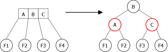
For a 3-node, there are two possibilities. Indeed, after an insertion and a rotation of rebalancing, the 3-node can be leaned to the left or leaned to the right as shown in Figure 26.

Figure 26. Transformation of a 3-node (leaned to the left or to the right)

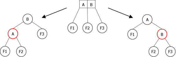
Remark: As there can never be two consecutive red links (links to red child) and that the branches have a number of black links equal to the height of the initial tree 2.3.4, the height of the tree is at most twice the height of the initial tree 2.3.4.

Remark 2: A red-black tree associated to a tree 2.3.4. of n elements has a height which is a logarithmic function of n.

Figure 27. Red-black tree associated to the tree 2.3.4 of figure 16

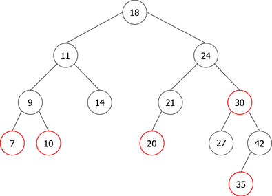
The figure 27 shows a possibility of red-black tree associated to the figure 16 tree. Indeed, a different data sequence (depending on eventual rebalancings) would give another tree with, for instance, 3-nodes leaned in the other way.

Searching in a red-black tree

In fact, regardless of the color of the nodes, it is a binary search tree and the search is done using search algorithms on ABR. So in the worst case the number of comparisons is logarithmic.

Insertion in a red-black tree

The insertion of an element can be done simulating the Insertion with splitting in going down. The splitting of a 4-node returns to invert the colors of the nodes as shown in Figure 28.

Figure 28. Splitting simulation of a 4-node in red-black representation

Unfortunately this transformation can create consecutive red nodes in the tree. This has the effect of unbalancing the tree. Therefore it must be rebalanced, and for this we will use the rotations seen previously.

Several cases may occur:

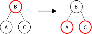
• The 4-node to split is linked to a 2-node. A simple inversion of the colors will be sufficient (Figure 29).

Figure 29. Splitting of a 4-node linked to a 2-node

• The 4-node to split is linked to a 3-node. We will assume that the 3-node is leaned to the right. In this case there are 3 possibilities:

• • It is the first child of the 3-node. There it is again sufficient to invert the colors (Figure 30).

Figure 30. Splitting of a 4-node linked to the first child of a 3-node leaned to the right

• • It is the second child of the 3-node. The inversion of the colors leads to an imbalance, it is sufficient to use a right-left rotation to rebalance the tree (Figure 31).

Figure 31. Splitting of a 4-node linked to the second child of a 3-node leaned to the right

• • It is the last child of the 3-node. The inversion of the colors leads to another imbalance, it is sufficient to use a left rotation to rebalance the tree (Figure 32).

Figure 32. Splitting of a 4-node linked to the last child of a 3-node leaned to the right

Remark: Obviously, there exist the three symmetric cases when the 3-node is leaned to the left.

Algorithm

The principle is simple, we descend from the root to the leaf where the new element has to be inserted. On this way, whenever a black node with two red children is met, we inverse their colors (split of the node). In this case, we must look if the parent of this node is not red in which case it is necessary to perform the appropriate rotation to rebalance the tree. Once the addition of the element is done, we must look if its parent is red. If this is the case, a rotation is also necessary. Indeed, the new leaves are systematically red in so far we add a twin element.

In terms of implementation, each node has to contain its own color. So, it is necessary to add a new field col taking the {Red, Black} values in the type record t_Node defined for the pointer-based implementation of the binary trees. That gives:

Types

   t_element = ...                /* Definition of the element type */
   color = (Red, Black)
   t_rbt = $\uparrow$t_rbtnode             /* Definition of the t_rbt type (pointer on t_rbtnode) */
   t_rbtnode = record             /* Definition of the t_rbtnode type */
      color     col
      t_element elt
      t_rbt     lc, rc
   end record t_rbtnode

Variables

   t_rbt rbtree

Remark: We will stay in the abstract formalism. For that we will use the rbt abstract type which is derived from the binarytree abstract type to which we added the specific operations to the Red-black trees, such as color that allows us to know the color of a node.

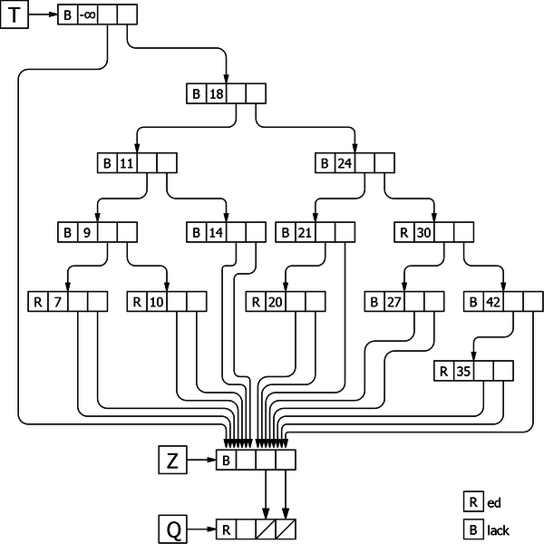
To simplify the algorithm, the insertion procedure uses a red-black tree with three extra elements: a head T, a sentinel Z and an element Q pointed by the sentinel as shown in Figure 33.

The head T contains an element whose value is less than all the possible others, its color is black, its left child points to the sentinel Z and its right child points to the root node if it exists. Its usefulness consists in avoiding the specific case of the insertion in an empty tree.

The sentinel Z is classical. All the tree nodes that must point to an empty tree, point to it. At the beginning, we assign it the value to add, which allows to avoid to test the two searching exit possibilities: the empty tree and the already existing element. Its color is black.

The element Q, for its part, allows to have only one processing, whether the color inversion takes place in the middle of the tree or on the leaf that we just have added. Its color is red and its two children point to an empty tree.

Figure 33. Representation (used by the algorithm of insertion) of the red-black tree of figure 27

algorithm procedure insertRBT
global parameters
   rbt     T, A
   boolean b
local parameters
   element x
   rbt     Z, Q
variables
   rbt     P, GP, GGP          /* Memorization of the three direct ascendants */
begin
   A $\leftarrow$ T
   Content(root(Z)) $\leftarrow$ x
   b $\leftarrow$ False
   P $\leftarrow$ T
   GP $\leftarrow$ T
   do
      GGP $\leftarrow$ GP
      GP $\leftarrow$ P
      P $\leftarrow$ A
      if x < content(root(A)) then
         A $\leftarrow$ l(A)
      else
         A $\leftarrow$ r(A)
      endif
      if color(l(A)) = Red and color(r(A))=Red then          /* 2 red children */
         if A = Z then          /* Insertion */
            b $\leftarrow$ True
            A $\leftarrow$ <Red,x,Z,Z>          /* Node creation, Col=Red */
            if x < content(root(P)) then
               l(P) $\leftarrow$ A
            else
               r(P) $\leftarrow$ A
            endif
         else
            color(A) $\leftarrow$ Red
            color(l(A)) $\leftarrow$ Black
            color(r(A)) $\leftarrow$ Black
         endif
         if color(P) = Red then          /* Rebalancing */
            si content(root(P)) > content(root(GP)) then
               si content(root(A)) > content(root(P)) then
                  LR(GP)
               else
                  RLR(GP)
               endif
            else
               if content(root(A)) > content(root(P)) then
                  LRR(GP)
               else
                  RR(GP)
               endif
            endif
            if content(root(GGP)) > content(root(GP)) then
                l(GGP) $\leftarrow$ GP
            else
               r(GGP) $\leftarrow$ GP
            endif
            color(GP) $\leftarrow$ Black          /* Color restoration */
            color(l(GP)) $\leftarrow$ Red
            color(r(GP)) $\leftarrow$ Red
            P $\leftarrow$ GP          /* hierarchy restoration */
            GP $\leftarrow$ AGP
            if x = content(root(P)) then
               A $\leftarrow$ P
            else
               if x < content(root(P)) then
                  A $\leftarrow$ l(P)
               else	
                  A $\leftarrow$ r(P)
               endif
            endif
         endif          /* End of rebalancing */
      endif          /* End of 2 red children */
   while x <> content(root(A))
   color(r(T)) $\leftarrow$ Black          /* Root always Black */
end algorithm procedure insertRBT

Conclusion

Regarding the different types of search trees, the complexity of search algorithm, of insertion algorithm and of deletion algorithm is always, at worst, bounded by a logarithmic function of the number of elements. As regards the average complexity order, we only have, in many cases, an experimental value. That said, we must consider the cost of reorganization (splitting, rotation) for insertion and deletion. An extreme case is the deletion of an element in an AVL which can cause up to $1.5 log_2^n$ rotations.

---

(Christophe "krisboul" Boullay)