Epita:Algo:Course:Sup-Info: Basic Searching Algorithms

Searching is one of the most fundamental and widely encountered problems in computer science. Given a collection of objects, the goal of searching is to find a particular object in this collection or to recognize that the object does not exist in the collection.

Often the objects have key values that are used for search and data values which correspond to the information one wishes to retrieve once an object is found. For example, a telephone book is a collection of names (on which one searches) and telephone numbers (which correspond to the data being sought).

For the purposes of this handout, we shall consider only searching for key values (e.g., names) with the understanding that in reality, one often wants the data associated with these key values.

The collection of objects is often stored in a list or an array. Often, the objects are sorted by key value (e.g., a phone book), but this need not be the case. Different algorithms for search are required depending whether the data is sorted or not. In what follows, we will describe some of them.

Definitions

A search is called associative search when the search criteria cover only the key value of the item.

A search is called positive search when the sought key is present in the data collection.

A search is called negative search when the sought key doesn't exist in the data collection.

Linear search (sequential search)

This search is extremely simple and suitable for collections of small data. Unless this is always the same elements that we search and that , in this case, we have adapted the list.

In an unordered list

Suppose that the given list is not necessarily sorted. This might correspond, for example, to a collection of exam scores which have not yet been sorted alphabetically. If a student wants to obtain his exam score, how does he do it ? he has to search through the entire collection of exams, one-by-one, until his exam is found. This corresponds to the unordered linear search algorithm.

The algorithm is the simplest possible. The sought key is compared item by item (sequentially) within the list. If one has a list l of n elements within which we search an element x and if we consider a Boolean function returning true if the search is positive and false if it is negative, we obtain the following algorithm:

Algorithm function search : boolean
Local parameters
   list     l
   element  x
Variables
   integer  i
Begin
   i $\leftarrow$ 1
   while i <= length(l) do            /* Number of elements of the list */
      if x = nth(l,i) then
         return(True)                 /* Positive search*/
      endif
      i $\leftarrow$ i + 1
   endwhile
   return(False)                      /* Negative search*/
End algorithm function search

In the worst case, we have to search through the entire list to get the final answer. That means we have to execute n comparisons. In this case, the worst-case, the complexity order is O(n) (see the lists). The average-case complexity is given by the probability that the x element is at the i-th position of the list. Unfortunately we do not know, in general, the positioning probability of the different elements. So we will ensure that those that are searched most frequently are at the beginning of the list.

Self organizing search

For lists that do not have a set order requirement, a self organizing algorithm may be more efficient if some items in the list are searched for more frequently than others. By shifting a found item toward the front of the list, future searches for that item will be executed more quickly.

This search is an adaptation of the previous. It can be applied only on unordered lists because it modifies the organization of the elements depending on the searches. There exist several possible ways:

• The agressive way: Each time an item is found, we put it directly at the first position of the list. This manner is only reasonably applicable to lists represented as linked-list because an array representation would shift all the elements located between the front and the one we found. The problem is putting infrequently sought elements in the first places.

• The soft way: Whenever we find an element, we shift it one place to the beginning of the list. This method is easily applicable to both forms of representation (array or linked list) since it is in fact a exchange of values. The problem is that searched elements advance too slowly: 2000 searches will be necessary to put a searched element located at the 2001^st position to make it reach the top of the list.

• the most suitable way: Whenever we find an element, we shift it an arbitrary number of places to the beginning of the list (for example, half of the distance between it and the first element). This method is easily applicable to the array implementation and has two advantages: first, the progression of a searched element to the beginning position is fast enough and so there will be no once searched item at the beginning of the list. In this case, the linked list implementation is the most suitable. Indeed, it is enough to have a pointer that progresses more slowly than the one of search (two times less in the case of half the distance) to know at every moment where will be the new position of the searched element.

In an ordered list

The algorithm and its complexity is the same as for the unordered list but with an advantage for negative searching. Indeed, the elements are ordered, it is easy to know if you have exceeded a value to find the searched element. Imagine a numeric list sorted in increasing order. We are looking for 12 and the list consists of elements {1,2,3,6,9,11,13,15,21,38,42}. When we arrive on the element 13, we are sure of not being able to find 12. That said, the worst complexity remains the same (searching for something bigger than the last).

The algorithm lightly modified gives:

Algorithm function search : boolean
Parameters locaux
   list    l
   element  x
Variables
   integer i
Begin
   i $\leftarrow$ 1
   while (i <= length(l)) et (x < nth(l,i)) do   /* Number of elements of the list */
      if x = nth(l,i) then
      return(True)                   /* positive search */
      endif
      i $\leftarrow$ i + 1
   endwhile
   return(False)                     /* negative search */
End algorithm function search

binary search

This requires that the list of items is sorted. In addition it is only applicable on an array implementation of the list. Assume a list l, a searched element x, and m the median position of the list, the principle of binary search is as follows:

• x = nth(l,m) then we have found x (the element we were looking for) and the search terminates successfully, returning position(m)

• x < nth(l,m) then x, if it exists, is located before the m^th and we recurse on the first half of the array, that is, on the range of ranks from 1 to m - 1

• x > nth(l,m) then x if it exists is located after the m^th and we recurse on the second half of the array, that is, on the range of ranks from m + 1 to length(l)

The search continues thus on a half subarray of elements after each comparison. If the search ends with an empty list, it means that the element x doesn't exist and that the search is negative.

The Binary search algorithm (recursive version), returning an integer value corresponding to the position on the list of the searched integer if it exists and 0 if not, is as follows:

algorithm function binary_search : boolean
Local parameters
   list    l
   element x
   integer left,right              /* left and right bounds of the list l */
Variables
   integer m                       /* median rank of the list l */
Begin
   if left <= right alors
      m $\leftarrow$ (left + right) div 2
      if x = nth(l,m) then
         return(m)                /* Positive search */
      else
         if x < nth(l,m) then
            return(binary_search(l,x,left,m-1))
         else
            return(binary_search(l,x,m+1,right))
         endif
      endif
   else
      return(0)                    /* Negative search*/
   endif 
End algorithm function binary_search

Remark: To search on the entire list, it is necessary to give, respectively, the value 1 and length(l) to left and right parameters.

The same algorithm in an iterative version:

Algorithm function iterative_binary_search : boolean
Local parameters
   list     l
   element  x
   integer  left,right             /* left and right bounds of the list l */
Variables
   integer   m                     /*  median rank of the list l */
Begin
   while left <= right do
      m $\leftarrow$ (left + right) div 2
      if x = nth(l,m) then
         return(m)                 /* Positive search */
      else
         if x < nth(l,m) then
            right $\leftarrow$ m - 1
         else
            left $\leftarrow$ m + 1
         endif
      endif
   endwhile
   return(0)                       /* Negative search */
End algorithm function iterative_binary_search

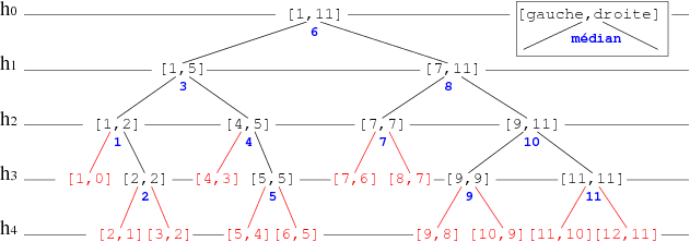
A representation of the execution of this algorithm applied to a sorted list of 11 elements may be given by using the decision tree learning shown in Figure 1. Each node represents a range of research: left and right bounds and the rank calculated from the median (blue). If the element is in this place the search ends positively, otherwise it continues on the appropriate axis (left or right depending on whether the desired value is smaller or larger than the median rank. If bounds intersect (range shown in red) the search ends negatively.

Remarks:

• Decision tree learning is a method commonly used in data mining. The goal is to create a model that predicts the value of a target variable based on several input variables.

• In the previous example each interior node corresponds to one of the indexes of the variables. These Indexes calculated represent all possible positions of the list. So if the element exists, it can not escape us (Gnark! Gnark! Gnark!).

• Each leaf represents a negative search range.

Figure 1. Decision tree learning of a binary search on a 11 element list.

This representation allows us to easily analyze the number of comparisons made by binary search. In fact, the algorithm traverses a branch, and ends (at worst) in an undefined range. In the case of positive search, the number of comparisons is equal to 2*height(v) where v is the node which corresponds to the index of the searched element. The tree being balanced, the height is bounded by $log_2^n$ where n is the power of 2 greater than or equal to the number of elements in the list. For our example of 11 elements $log_2^{16} = 4$.

binary search of the first occurrence of an element

In case the list has several occurrences of the elements, it can be interesting to want a specific one. Suppose it is the first occurrence we are looking for. It is essential to maintain the binary search principle rather than a sequential search when we are on any occurrence of the element. Indeed, the full benefit of the binary search could be lost because of the distance of the first occurrence compared to the one on which we find ourselves. Therefore, we will modify the iterative version of the binary search and apply necessary changes. Then we obtain iteratively:

Algorithm function iterative_firstocc_binary_search : boolean
Local parameters
   list     l
   element  x
   integer  g,d                    /* left and right bounds of the list l */
Variables
   integer  m                      /* median rank of the list l */
Begin
   while left < right do
      m $\leftarrow$ (left + right) div 2
      if x < ième(l,m) then
         right $\leftarrow$ m - 1
      else
         left $\leftarrow$ m + 1
      endif
   endwhile
   if x = ième(l,g) then           /* g ou d */
      return(m)                    /* Positive search */
   else
      return(0)                    /* Negative search */
   endif
End algorithm function iterative_firstocc_binary_search

Linear interpolation search

The linear interpolation search also requires a sorted list in array implementation. Its principle is similar to the binary search. The difference lies in the calculation of the index of the element. The binary search uses a median element, the linear interpolation search calculates the position by considering the arrangement of data.

For instance, when you look in a dictionary for the word "peanuts", you do not open the dictionary in the middle, but at the end, where you think you have the best chance to find the word "peanuts". This is the principle of the linear interpolation search: Estimate the probable position of the item.

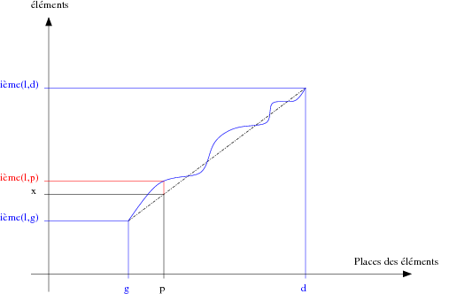
Assume a data list l sorted in increasing order. Suppose the progression of these data is linear. When searching the element x between left bound left and right bound right, it seems interesting to see at the p position defined by p = left + ((right - left) * (x - nth(l,left) div (nth(l,right) - nth(l,left)) if x is here, as in the example in Figure 2.

Figure 2. Example of linear interpolation search.

This function is the ratio of the distances between, on the one hand, the left, the right, and the x elements of the list l and on, the other hand, the left and right bounds and the estimated position of the element x of the list l (The intercept theorem, also known as Thales' theorem).

As shown in the example of Figure 2, we have the true distribution function of the elements of the list l shown in blue. Assume the position of the desired element x is the interpolated position p based on a linear distribution function (dashed black line). The question is to know if the p ^th element of l is equal to x. In this example, it is clear that it is not.

As for the binary search principle, this method uses the fact that a list is sorted. In addition it is only applicable on array representation of list. Assume a list l, a searched element x, and the estimated place p of the searched element, the principle of linear interpolation search is as follows:

• x = nth(l,p) then we have found x (the element we were looking for) and the search terminates successfully returning position(p)

• x < nth(l,p) then x if it exists is located before the p^th and we recurse on the first half of the array, that is, on the range of ranks from 1 to p - 1

• x > nth(l,p) then x if it exists is located after the p^th and we recurse on the second half of the array, that is, on the range of ranks from p + 1 to length(l)

The search continues thus on a half subarray of elements after each comparison. If the search ends with an empty list, it means that the element x doesn't exist and that the search is negative.

The linear interpolation search algorithm (recursive version), returning an integer value corresponding to the position on the list of the searched integer if it exists and 0 if not, is as follows:

Algorithm function linear_interpolation_search : boolean
Local parameters
   list     l
   element  x
   integer  left,right             /* left and right bounds of the list l */
Variables
   integer  p                      /* estimated position of the searched element */
Begin
   if left <= right then
      p $\leftarrow$ left + ((right - left) * (x - nth(l,left) div (nth(l,right) - nth(l,left))
      if x = nth(l,p) then
         return(p)                 /* Positive search */
      else
         if x < nth(l,p) then
            return(linear_interpolation_search(l,x,left,p-1))
         else
            return(linear_interpolation_search(l,x,p+1,right))
         endif
      endif
   else
      return(0)                    /* Negative search */
   endif 
End algorithme function linear_interpolation_search

The same algorithm in an iterative version:

Algorithm function interative_linear_interpolation_search : boolean
Local parameters
   list     l
   element  x
   integer  left,right             /* left and right bounds of the list l */
Variables
   integer  p                      /* estimated position of the searched element */
Begin
   while left <= right do
      p $\leftarrow$ left + ((right - left) * (x - nth(l,left) div (nth(l,right) - nth(l,left))
      if x = nth(l,p) then
         return(p)                /* Positive search */
      else
         if x < nth(l,p) then
            right $\leftarrow$ p-1
         sinon
            left $\leftarrow$ p+1
         endif
      endif
   endwhile
   return(0)                      /* Negative search*/
End algorithm function interative_linear_interpolation_search

Remarks:

• The difficulty in relation to binary search is to give a good interpolation function. The ideal is to have a uniform distribution function of elements in the list. In Complexity words, if n is the number of elements in the list, the order of the binary search is about $log_2^n$ and the linear interpolation (if the distribution is uniform) is about $log_2^{log_2^n}$

• This seems much more interesting than the binary search, but there is a drawback: it requires that the data in the list are numerics or quickly numerisable. Indeed, we use the value of the searched element in the calculation of the estimated position, which is not the case for the binary search. It induces a waste of time that is not necessarily negligible. In addition, to make it interesting it is necessary that the list be very large, so that the difference between $log_2^{log_2^n}$ and $log_2^n$ is sufficiently large.

---

(Christophe "krisboul" Boullay)