Epita: Algo: Course: Info-Spe: shortest path algorithms
Contents |
Overview
Remarks and definitions:
- We will focus on the non zero-length paths.
- We will work with edge-weighted directed graphs.
- The cost (weight or value) of a path is equal to the sum of the cost of the arcs that compose it. We call it the distance of the path.
- The shortest path from a vertex x to a vertex y is the minimum cost path from x to y. Such a path does not necessarily exist.
- The shortest distance from a vertex x to a vertex y is the cost of the shortest path if it exists.
Conditions of existence:
Consider a path M from a vertex x to a vertex y. Suppose this path contains a circuit T. Call M' the obtained path removing T of M. We then have the following cost relation:
Cost(M) = Cost(M') + Cost(T)
If the Cost(T) is negative (<0), there exists no shortest path from x to y. Indeed, it is sufficient to simply cross the circuit T again to get a better result (lower cost path).
Such a circuit is called negative (directed) cycle.
If the Cost(T) is zero (=0), M' has the same cost than M. In this case it is also a shortest path but its length (number of vertices crossed) is greater than the one of M.
If the Cost(T) is positive (>0), the Cost of M' is less than the one of M. In this case it is a better candidate than M for the shorstest path.
If there exist circuits, their cost is positive or zero. But a shortest path can not contain a positive cost circuit and if there exist nul cost circuits, there are several solutions to the problem.
Since the number of elementary paths (in which all vertices are distinct) from a vertex x to a vertex y is finite, there exists at least one elementary shortest path from x to y (remark: There may be several).
In conclusion: There exists a solution to the shortest path problem from x to y if there exists a path from x to y and there is no negative cycle.
Variants of the problem:
The algorithms we present give, in the case where there is no negative cycle, un elementary shortest path.
The three ways of searching for a shortest path are:
- between two vertices x and y,
- from a vertex x (a source) to all the other vertices of the graph,
- between all pairs of vertices x and y.
Remarks:
- The 1) is considered as the best solution of the 2), we focus only on the 2) and 3).
- There is no general algorithm for the 2) nor for the 3). It is necessary to consider the properties of the manipulated graphs and the problem posed and then choose the most suitable algorithm.
Dijkstra
The Dijkstra algorithm is usable only in the very frequent cases where the cost of the arcs are positive or zero. It determines the shortest path between a source vertex x and all the other vertices of the graph reachable from x. Then we obtain a tree of root x formed by the shortest paths from x to the vertices reachable by x. It should be noted that, having no negative costs, it accepts graphs containing circuits.
Principle
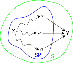
Let G=< S,A,C > be a weighted directed graph of n vertices. Let x be a vertex of S. It is proposed to build a set SP (shortest path) of vertices y for which the shortest path from x is known.
- Initially, SP only contains the source (x).
- At each step a vertex y, for which the smallest distance (sdistance(x,y,G)) and the parent (parent(x,y,G)) are known, is added to SP.
- We stop when SP contains all vertices reachable from x.
Let M be the complement set of SP in S (M=S-SP) and for all vertices y of M, we call path from x to y in SP any path from x to y having only vertices of SP except y (see figure 1.).
|
We write distancex,SP(y), the cost of the shortest path from x to y in SP and predx,SP(y) the predecessor of y in this shortest path.
At each step, we choose a vertex m of M such as:
distancex,SP(m) = Min{distancex,SP(y)} 
Algorithm
The algorithm traverses the graph g from a source vertex x and returns two arrays: sp and pr to memorize the shortest paths and their respective distance. sp[y] will memorize distancex,SP(y) and pr[y] will memorize predx,SP(y).
To avoid useless tests, we will extend the capabilities of the cost function to be defined for all pairs of vertices (x,y) as follows:
cost(x,x,g) = 0 for a graph without loop
cost(x,y,g) =if <x,y> isanarcof g = false
We will also use an operation choosemin(M, sp) which will return the vertex  such as sp[m] is minimum, and the operations on sets.
For the Dijkstra algorithm, the data type used are the following:
Constants

   Nbv = ...                           /* Vertices Number of the graph */

Types

   t_vectNbvReal = Nbv real            /* Vector of Nbv real */
   t_vectNbvInt  = Nbv integer         /* Vector of Nbv integer */
That gives:
Algorithm procedure Dijkstra Local parameters integer x /* x is the source vertex */ graph g Global parameters t_vectNbvReal sp /* sp[y] is the distance of the shortest path from x to y*/ t_vectNbvInt pr /* pr[y] is the predeécessor of y in this path */ Variables integer i, y, m /* y and m are vertices */ real v set M Begin /* Initialization */ Memptyset for i
1 to n do sp[i]
cost(x,i,g) pr[i]
x M
insert(i,M) endfor M
delete(x,M) /* SP={x} */ /* Successive insertions of vertices to SP */ while M <> emptyset do m
choosemin(M,sp) if sp[m] =
then /* no more reachable vertex from x */ return endif M
delete(m,M) /* insertion of m to SP */ /* adjustment of the distance values */ for i
1 to do+(m,g) do y
nthsucc(i,m,g) if y
M then /* the shortest path from x to y is not already determined */ v
sp[m] + cost(m,y,g) if v < sp[y] then sp[y]
v pr[y]
m endif endif endfor endwhile End algorithme procedure Dijkstra
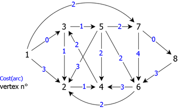
Apply the Dijsktra algorithm to the weighted directed graph of the figure 2 using the vertex 1 as source vertex (we search to determine the shortest paths from 1 to all the others.)
Remark: the vertices are treated in increasing order, whether in the set M or as successors.
|
After the execution of Dijkstra algorithm, we obtain the vectors sp and pr as follows (table 1):
| Vertices (index) | 1 | 2 | 3 | 4 | 5 | 6 | 7 | 8 |
| SP | 0 | 1 | 0 | 2 | 1 | 3 | 2 | 2 |
| PR | 1 | 3 | 1 | 2 | 3 | 5 | 1 | 7 |
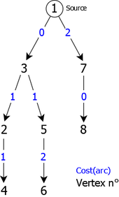
That corresponds to the tree of root 1 as follows (see Figure 3):
|
For instance, to know the shortest path from vertex 1 to vertex 4, it is sufficient to go back from vertex 4 (destination) to vertex 1 (the source) using vector pr, its cost (shortest distance) being obtained by sp[4], which gives:
shortest path from 1 to 4 : 13
2
4 of cost: 2
Bellman
The Bellman algorithm is usable in cases where the costs of the arcs are of any kind, but where the graph does not have a circuit. It determines the shortest path between a source vertex x (root of the graph) and all the other vertices of the graph reachable from x. Then we obtain a tree of root x formed by the shortest paths from x to the vertices reachable by x.
Principle
Let G=< S,A,C > be a weighted directed graph of n vertices. Let x be a vertex of S, we shall build a set SP (shortest path) of vertices y for which the shortest path from x is known. Let M be the complement set of SP in S (M=S-SP). M is the set of vertices y for which sdistance(x,y,G) is not already known.
We can calculate sdistance(x,y,G) only when all the predecessors of y are in SP.
 it is necessary to know its indegree (number of predecessors) and to be able to access to its ith predecessor.
The idea is as follows:
A shortest path from x to y must pass by m, one of the predecessors of y (see figure 4). The predecessor for which sdistance(x,m,G) + cost(m,y,G) is minimum.

|
Algorithm
The algorithm returns two arrays: sp and pr to memorize the shortest paths and their respective distance. sp[y] will memorize distancex,SP(y) and pr[y] will memorize predx,SP(y).
To avoid useless tests, we will extend the capabilities of the cost function to be defined for all pairs of vertices (x,y) as follows:
cost(x,x,g) = 0 for a graph without loop
cost(x,y,g) =if <x,y> isanarcof g = false
- Initially, SP contains only the source (x).
- At each step the algorithm chooses in M a vertex y for which all predecessors are in SP. We search by which of its predecessors the path from x is the shortest. Then this vertex is added to SP and the vectors sp and pr are updated.
- We stop when M is empty.
We will use the operation choosenext(M, g) which will return the vertex  that has no more predecessors in M.
For the Bellman algorithm, the data type used are the following:
Constants

   Nbv = ...                           /* Vertices Number of the graph */

Types

   t_vectNbvReal = Nbs real            /* Vector of Nbv real */
   t_vectNbvInt  = Nbs integer         /* Vector of Nbv integer */
That gives:
Algorithm procedure Bellman Local parameters integer x /* x is the source vertex */ graph g Global parameters t_vectNbvReal sp /* sp[y] is the distance of the shortest path from x to y*/ t_vectNbvInt pr /* pr[y] is the predeécessor of y in this path */ Variables integer i, y, z, m /* y, z and m are vertices */ real min, aux /* min and aux are distances */ set M Begin /* Initialization */ Memptyset for i
1 to n do M
insert(i,M) endfor M
delete(x,M) /* SP={x} */ sp[x]
0 pr[x]
x /* Successive insertions of vertices to SP */ while M <> emptyset do m
choosenext(M,g) M
delete(m,M) /* insertion of m to SP */ y
nthpred(1,m,g) /* First predecessor and its associated distance */ min
sp[y] + cost(y,m,g) /* comparison with the other predecessors */ for i
2 to do-(m,g) do z
nthpred(i,m,g) /* ith predecessor and its associated distance */ aux
sp[z] + cost(z,m,g) if aux < min then /* the shortest path from x to y is not already determined */ min
aux y
z endif endfor sp[x]
min pr[x]
y endwhile End algorithm procedure Bellman
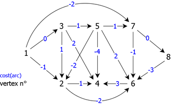
Apply the Bellman algorithm to the weighted directed graph of figure 5 using the vertex 1 as source vertex (We are trying to determine the shortest paths from 1 to all the others.)
Remark: the vertices are treated in increasing order, whether in the set M or as successors.
|
After the execution of Bellman algorithm, we obtain the vectors sp and pr as follows (table 2):
| Vertices (index) | 1 | 2 | 3 | 4 | 5 | 6 | 7 | 8 |
| SP | 0 | -1 | 0 | -3 | 1 | -5 | -2 | -2 |
| PR | 1 | 5 | 1 | 5 | 3 | 8 | 1 | 7 |
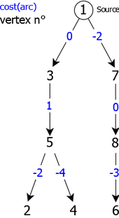
That corresponds to the tree of root 1 as follows (see Figure 6):
|
For instance, to know the shorstest path from vertex 1 to vertex 4, it is sufficient to go back from vertex 4 (destination) to vertex 1 (the source) using vector pr, its cost (shortest distance) being obtained by sp[4], which gives:
shortest path from 1 to 4 : 13
5
4 of cost: -3
Floyd
The Floyd algorithm is usable in cases where the costs of the arcs are of any kind, with or without circuit but without negative circuit. It determines the shortest path between all pairs of vertices (x,y) of a graph G.
We can use the Bellman or the Dijkstra algorithms by varying the root, but not for graphs with any costs and having non negative circuits.
The Floyd algorithm is one of simple algorithms which determine all the shortest paths using a matrix representation.
Principle
The principle of this algorithm is the same as The Warshall algorithm used to determine the transitive closure of a graph (connectivity of the graph).
Let G=< S,A,C > be a weighted directed graph of n vertices.
- Initially, we consider only the paths x to y that do not go through other vertices of the graph. Then we have sdistance(x,y,G) = cost(x,y,G) an parent(x,y,G) = x.
- At each step i, we calculate distancei(x,y) the cost of the shortest path from x to y going through vertices that are less or equal to i. If this distance is less than the current known shortest distance, it becomes this shortest distance and parent(i,y,G) replaces parent(x,y,G).
Algorithm
The algorithm will use two matrices: sp and pr to memorize the shortest paths and their respective distance. sp[x,y] will memorize sdistancei(x,y) and pr[x,y] will memorize parenti(x,y).
To avoid useless tests we will extend the capabilities of the cost function to be defined for all pairs of vertices (x,y) as follows:
cost(x,x,g) = 0 for a graph without loop
cost(x,y,g) =if <x,y> isanarcof g = false
- Initially sp and pr are respectively initialized by cost(x,y,G) and x.
- At each step i, these two matrices are updated by some possible shortest paths encountered going through vertices less than or equal to i.
For the Floyd algorithm, the data type used are the following:
Constants

   Nbv = ...                                   /* Vertices Number of the graph */

Types

   t_matNbvNbvReal = Nbv x Nbv real            /* Square matrix of Nbv real */
   t_matNbvNbvInt  = Nbv x Nbv integer         /* Square matrix of Nbv integer */
That gives:
Algorithm procedure Floyd local parameters graph g global parameters t_matNbvNbvreal ppd /* Adjacency matrix of the graph g */ t_matNbvNbvint pr /* Adjacency matrix of the graph g* */ Variables integer i, x, y /* i, x and y are vertices */ begin /* Initialization of sp and pr */ for x1 to Nbv do for y
1 to Nbv do sp[x,y]
cost(x,y,g) pr[x,y]
x endfor endfor
/* Calculation of the shortest paths */ for i1 to Nbv do for x
1 to Nbv do for y
1 to Nbv do if sp[x,i] + sp[i,y] < sp[x,y] then sp[x,y]
sp[x,i] + sp[i,y] pr[x,y]
pr[i,y] endif endfor endfor endfor end algorithm procedure Floyd
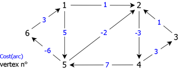
Apply the Floyd algorithm to the weighted directed graph of the figure 7.
|
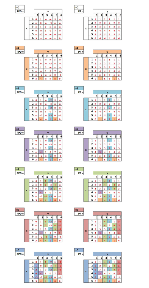
After running the Floyd algorithm, we obtain the matrices sp and pr as follows (table 3):
|
For instance, to know the shortest path from vertex 6 to vertex 3, it is sufficient to go back from vertex 3 (destination) to vertex 6 (the source) using vector pr, its cost (shortest distance) being obtained by sp[6,3], which gives:
pr[6,3] (4)
pr[6,4] (2)
pr[6,2] (1)
pr[6,1] (6)


The the shortest path from 6 to 3 is: 6 -> 1 -> 2 -> 4 -> 3 of cost sp[6,3]: 4
(Christophe "krisboul" Boullay)