Epita: Algo: Course Info-Spe: the minimum spanning tree

Overview

Remarks and recalls:

• The cost (weight or value) of a path is equal to the sum of the cost of the edges that compose it and will for a graph G be noted Cost(G).
• The following properties are, for a graph G = < S, A, C > of n vertices, specific of a tree and are all equivalents:
  • G is acyclic and connected.
  • G is connected with n-1 edges.
  • G is connected but removing any edge disconnects it (any edge is an isthme).
  • G is acyclic with n-1 edges.
  • G is acyclic but adding any edge creates a cycle.
  • Each pair of vertices {x,y} of S is joined by a unique chain of G.

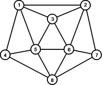
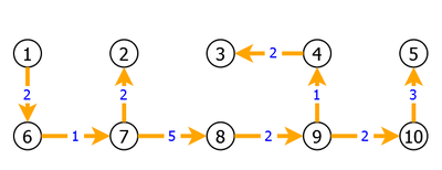
A ST (Spanning Tree) is obtained, for a connected graph G, building a partial graph of G that is a tree. that is to say connected and acyclic. We can see in figure 1 a connected graph with two possible examples of spanning tree.

Figure 1. A non weighted connected graph and two possible spanning trees.

Original Graph	Spanning Tree	Spanning Tree

Conditions of existence:

Suppose a weighted non-directed connected graph G = < S, A, C>. The spanning tree problem consists to find a partial graph of G which is connected and whose cost is minimum. Such a graph can not have a cycle, otherwise the deletion of one of its edges would give a graph with a less cost and a best spanning tree candidate. As it is connected it is a tree and whose cost is minimum.

Remark: However if the graph G is not connected, it is always possible to determine a partial acyclic graph of G. We then obtain a spanning forest constituted by as many trees as there is connected components in the graph G.

A simple way to determine a spanning tree is to remove from the original graph all edges forming cycles. The number of spanning trees being finite, we are sure to find one of minimum cost.

Question: Does this ST be unique?

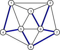
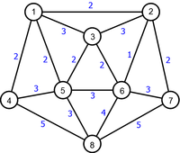
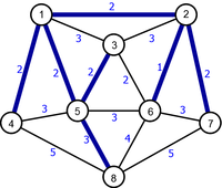
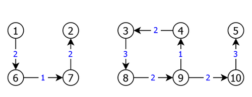
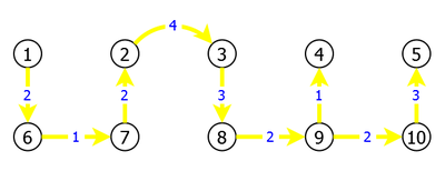
Generally not, as we can see in Figure 2 which shows two possible examples of MST (Minimum Spanning Tree). On the other hand, if the cost of the edges are all distinct, we can show that the MST obtained is unique.

Figure 2. A weighted connected graph and two minimum possible spanning trees.

Original Graph	Minimum Spanning Tree	Minimum Spanning Tree

Variants of the problem:

We will consider the two most classical algorithms:

1. Prim which like Dijkstra on the principle is useful for sparse graphs, maintains the connection of all the edges of the tree in construction,
2. Kruskal which is very effective on dense graphs, focuses on maintaining acyclicity of the graph in construction.

Prim

As said earlier, Prim algorithm is very close to Dijkstra Algorithm. We start from a vertex (the source) and then at each iteration we choose the free nearest vertex (in terms of weight) while maintaining the tree property (acyclic and connected).

Principle

Let G = < S, A, C > be a undirected weighted graph of n vertices. We propose to build a tree T (partial graph of G).

Let x be a vertex of S. Call SC the set of vertices y connected to x in T and SR its complement set in S, that is to say the set of vertices of S remaining to connect to x.

• Initially, SC only contains the source (x).
• At each step a vertex y of SR, such as the cost of the edge {x,y} is minimum, is added to SC. This reflects the addition of the edge {x,y} in T.
• We stop when SR is empty (SC = S).

Remark: if the graph G is not connected, we stop when SC contains all vertices reachable from x.

The choice of the edges being that both vertices belong to two complementary sets, guarantees us the absence of cycle. In addition the cost of the choosen edge being minimum, we are also assured that the cost of the obtained tree T is minimum. Therefore it is an MST.

Algorithm

The algorithm traverses the graph g from a source vertex x and returns a graph t corresponding to the builded MST. To do this we wil use two tables: nv and c to memorize for each vertex the nearest vertex connecting it to x and the cost of the edge between these two vertices. That is to say that nv[y] will memorize the edge { y, nv[y] } and c[y] will memorize cost( y, nv[y], g ).

To avoid useless tests, we will extend the capabilities of the cost function to be defined for all pairs of vertices (x,y) as follows:

cost(x,x,g) = 0 for a graph without loop


cost(x,y,g) = $\infty$ if <x,y> isanedgeof g = false

We will also use an operation choosemin(SR, c) which will return the vertex $m\in SR$ such as c[m] is minimum, and the operations on sets.

For the Prim algorithm, the data type used are the following:

Constants

   Nbv = ...                           /* Vertices Number of the graph */

Types

   t_vectNbvReal = Nbv real            /* Vector of Nbv real */
   t_vectNbvInt  = Nbv integer         /* Vector of Nbv integer */

That gives:

Algorithm procedure Prim
Local parameters
   integer x                           /* x is the source vertex */
   graph g
Global parameters
   graph t                             /* t is the mst we are building */
Variables
   t_vectNbvInt  nv                    /* nv[y] is the nearest vertex of y */
   t_vectNbvReal c                     /* c[y] is the cost of the edge between y and nv[y]*/
   integer i, y, z, m                  /* y and m are vertices */
   real v
   set SR
Begin
   /* Initialization */
   T $\leftarrow$ emptygraph
   SR $\leftarrow$ emptyset
   for i $\leftarrow$ 1 to n do
      c[i] $\leftarrow$ cost(x,i,g)
      nv[i] $\leftarrow$ x
      SR $\leftarrow$ insert(i,SR)
   endfor
   SR $\leftarrow$ delete(x,SR)                       /* SC={x} */
   while SR <> emptyset do                   /* Successive additions of edges to T */
      m $\leftarrow$ choosemin(SR,d)
      SR $\leftarrow$ delete(m,SR)                    /* addition of m to SC */
      z $\leftarrow$ nv[m]
      v $\leftarrow$ cost(m,z,g)
      t $\leftarrow$ addedge <m,z> weighted v to t
      /* adjustment of the distance values */
      for i $\leftarrow$ 1 to do(m,g) do
         y $\leftarrow$ nthbeighbor(i,m,g)
         if (y $\in$ SR)  and (cost(m,y,g)<c[y]) then  
            c[y] $\leftarrow$ cost(m,y,g)
            nv[y] $\leftarrow$ m
         endif
      endfor
   endwhile
End algorithme procedure Prim

Example

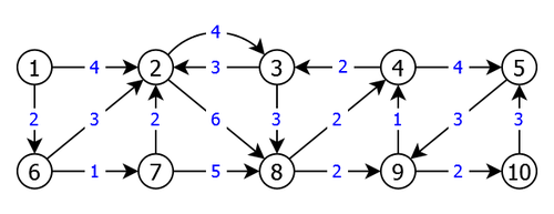
Apply the Prim algorithm to the weighted undirected connected graph in Figure 2 using the vertex 1 as source vertex.

Kruskal

The Kruskal algorithm is based on one property of trees, which says that a graph G of n vertices is a tree if it is acyclic with n-1 edges. We start from an empty graph and adding n-1 edges while respecting the tree property being 'acyclic'.

Principle

Let G = < S, A, C > be a undirected weighted connected graph of n vertices and p edges. We propose to build a tree T = < S, AC, C> (partial graph of G).

Let {x,y} be an edge of A. Call AC the set of the choosen edges and AR its complement set in A, that is to say the set of remaining edges of A.

• Initially, AC is empty.
• At each step an edge {x,y} of AR, such as the cost of this edge is minimum and does not create a cycle in T, is added to AC.
• We stop when we added n-1 without creating cycles.

Question: How knowing if the addition of the edge {x,y} to T creates a cycle or not ?

It is sufficient, for that, to know if it already exists in T a chain connecting x and y. That reflects the belonging of x and y to a same connected component of T. If this is not the case, adding the edge {x,y} joins the two components into one.

Algorithm

To do that the Kruskal algorithm uses:

• A table parent which associated to the functions find and union (cf connectivity of an undirected evolutive graph) allows us to know if two vertices x and y of the graph T belong to the same connected component or not. If it is the case that means that adding to T the edge {x,y} will create a cycle. What will not do the algorithm to keep the acyclicity property of a tree.

• a set U containing the weighted edges of the graph G (At start U=A).

At each turn the algorithm chooses the minimum cost edge of U. This latter is removed from U and, if it does not create cycles, it is then added to T and counted.

When n-1 edges were added, the graph T is constituted of the n-1 minimum cost edges not creating cycles. Therefore it is a MST of G.

We will use the operation choosemin(U) which will return the minimum cost edge {x,y,v} of U, and the set operations.

For the Kruskal algorithm, the data type used are the following:

Constants

   Nbv = ...                           /* Vertices Number of the graph */

Types

   t_vectNbvInt  = Nbv integer         /* Vector of Nbv integer */

That gives:

Algorithm procedure Kruskal
Local parameters
   graph g                             /* g is an undirected weighted graph */
Global parameters
   graph t                             /* t is the mst we are building */
Variables
   t_vectNbvInt  parent                /* parent is the ascendant vertex table */
   set U
   integer i, x, y, rx, ry             /* x, y, rx and ry are vertices */
   real v
Begin
   /* Initialization */
   t $\leftarrow$ emptygraph
   U $\leftarrow$ emptyset
   for x $\leftarrow$ 1 to n do
      parent[i] $\leftarrow$ -1
      for i $\leftarrow$ 1 to d°(x,g) do
         y $\leftarrow$ nthbeighbor(i,x,g)
         U $\leftarrow$ insert({x,y,cost(x,y,g)},U)
      endfor
   endfor
   i $\leftarrow$ 1                                       /* Number of choosen edges = 0 */
   /* Successive additions of edges to T */
   while i < n do                                /* While there is not n-1 edges */
      {x,y,v} $\leftarrow$ choosemin(U)                   /* choice of the new edge */
      U $\leftarrow$ delete({x,y,v},U)      
      rx $\leftarrow$ find(x,parent)
      ry $\leftarrow$ find(y,parent)
      /* Control of acyclicity */
      if (rx <> ry) then
         union(rx,ry,parent)
         t $\leftarrow$ addedge <x,y> weighted v to t
         i $\leftarrow$ i + 1                             /* one edge more */
      endif
   endwhile
End algorithm procedure Kruskal

Example

Apply the Kruskal algorithm to the weighted undirected connected graph in Figure 2.

Edmonds

The Edmonds algorithm has the feature to determine, starting from a source vertex, a Minimum Spanning Tree of a weighted directed graph.

Principle

Let G = < S, A, C > be a weighted directed graph with n vertices and p arcs, we then search a Minimum Spanning Tree (MST) T of fixed root r. The Edmonds algorithm will use the two following definitions of a Spanning Tree (ST) of G.

1. T is a spanning tree of G (if we forget the direction)
2. Any vertex of G has an unique predecessor, except the fixed root r that has no one.

These definitions lead us to write a heuristic that will build the spanning subgraph G' = < S, A', C> who can be a tree. The idea is to keep for each vertex y of G (except for the root vertex r) its closest predecessor x (the one for which the lowest cost incoming arc of the vertex), that gives :

Algorithm procedure heuristic_Build_Spanning_Subgraph 
Local parmeters
   integer r                        /* r is the root vertex */
   graph g
Global parameters
   graph g'                         /* the spanning subgraph under construction */
Variables
   integer x, y, m                  /* x, y and m are vertices */
   real v
Begin
   g' $\leftarrow$ emptygraph                 /* Initialization of g' */
   for y $\leftarrow$ 1 to n do
      if y<>r then
         m $\leftarrow$ nth-pred(1,y,g)
         v $\leftarrow$ cost(m,y,g)
         for i $\leftarrow$ 2 to do-(y,g) do
            x $\leftarrow$ nth-pred(i,y,g)
            if (cost(x,y,g)<v) then
               v $\leftarrow$ cost(x,y,g)
               m $\leftarrow$ x
            endif
         endfor
         g' $\leftarrow$ addedge <m,y> weighted v to g'
      endif
   endfor
End Algorithm procedure heuristic_Build_Spanning_Subgraph 

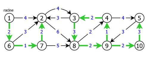
Apply this heuristic to the graph G = < S, A, C > of figure 3 using the vertex 1 as root.

Figure 3. A weighted directed graph containing a circuit and 2 connected components.

We would then have the spanning subgraph G' = < S, A', C> of figure 4:

Figure 4. Spanning subgraph of the graph of Figure 3 generated by the heuristic.

Once the heuristic applied to G:

• if G' is a tree, it is also a MST and it is over,
• if G' is not a tree, it has a cycle and it is not connected. Indeed a tree is connected without cycles with n-1 edges. The heuristic has retained one edge per vertex except for the chosen root of the graph (the vertex 1 in the example of Figure 3), which gives n-1 edges. So G' not being a tree, it is not connected and has at least one cycle, as shown by the application result figure 4.

Note: If G' has cycles, they are also circuits since all arcs are oriented in the same direction (otherwise a vertex has two predecessors). We then deduce the following property:

P1: If the spanning subgraph G'  builded by the heuristic is not a tree, it is not connected and has at least one circuit.

The Edmonds algorithm exploits the graph G' due to the following property:

P2: Let μ be one of the circuits of the spanning subgraph G'  generated by the heuristic, it exists a MST T which contains all the arcs of μ except one.

This property will allow us to contract the circuit μ into a single vertex called pseudo_vertex and continue searching our MST on the contracted graph.

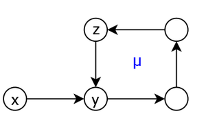
Let's call incoming arc in μ an arc (x,y) with the vertex y in μ and x not. Let's also call z the predecessor vertex of y in the circuit μ (see figure 5).

Figure 5. A circuit μ and an incoming arc (x,y).

Let G = < S, A, C > be a weighted directed graph and μ be a circuit. We call contracted graph G/μ = G₁ = <S₁, A₁> the graph obtained by replacing μ by a pseudo-vertex. The incoming edges to this pseudo-vertex are the incoming arcs in μ. After the contraction of μ, T then becomes a tree T₁ on G₁ whose weight is linked to that of T by the relation:

C(T) = C(T1) + C(μ) - C(z,y,G) with C the cost function of G

The costs C₁ of G₁ will be modified as follows:

• C₁(x,y,G₁) = C(x,y,G) if (x,y) is not an incoming arc in μ
• C₁(x,y,G₁) = C(x,y,G)-C(z,y,G) if (x,y) is an incoming arc in μ with z the predecessor of y in μ

THe aim of this cost modification is to finally have:

C(T) = C1(T1) + C(μ)

Which gives the following property:

P3: T is a MST of G iaoi it is also true for its restriction T1 in the contracted graph G1 = G/μ fitted with the costs C1.

Therefore we can apply the heuristic to G to compute G' . If this latter contains circuits, we contract them correcting the cost of their incoming edges. That gives the graph G₁ fitted with the costs C₁ on which the process (heuristic, possible contractions, etc) is repeated.

We then obtain a sequence of contracted graphs G_k with their spanning subgraph G'_k and we only stop this when the spanning subgraph G'_k of the graph G_k is a tree T_k.

If the graph G_k contains the contraction of a circuit μ of the graph G_k-1 and that G'_k (the spanning subgraph) is a tree T_k, we know, due to the property P₂, that this tree has an unique incoming arc (x,y) in μ. If z is the predecessor of y in the circuit μ, we tehn can rebuild the tree T_k-1 by adding to the tree T_k all the arcs of μ except (z,y).

This intermediate tree recovery operation is repeated from intermediate tree to intermediate tree until it finds the tree T of original graph G, what for Edmonds Algorithm would give the following structure:

G' $\leftarrow$ G
r $\leftarrow$ ...     /* choice of r the root vertex */
do
   T $\leftarrow$ heuristic_Build_Spanning_Subgraph (r, G')
   for each circuit μ of T do
      G' $\leftarrow$ contraction of G' on μ
      Modifications of the cost of the incoming arc in μ depending on the property P3
   endfor
while  T has a circuit.
Rebuild of the MST T of  G by successive recoveries of the intermediate trees

Example

Let's try to clarify all this with an example. Take the graph of figure 6 representing our graph G=G₀ and the spanning subgraph G'₀ obtained after the application of the heuristic.

Figure 6. The graph G=< S, A, C > and its spanning subgraph G'=< S, A', C >.

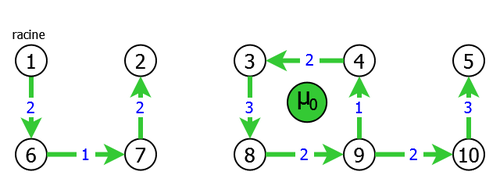
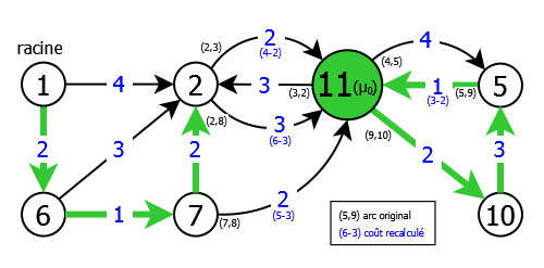
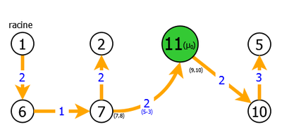
We then see that there are two components and a circuit μ₀ (3,8,9,4,3). So we will contract the graph G = G₀ on the circuit μ₀ by replacing this latter by a pseudo-vertex 11. We will then readjust the cost of the incoming arcs (2,3), (2,8), (7,8) and (5,9) in μ₀, and finally relaunch the heuristic on the obtained graph G₁ = G₀/μ₀ = < S₁, A₁, C₁ >, which gives (see. figure 7):

It should be noted that the contraction of a graph on a circuit can generate multiple arcs between two vertices, as it is the case in this example. Indeed there are two arcs (2,11) replacing the arcs (2,3) and (2,8) of the previous graph.

Figure 7. The graph G₁ = < S₁, A₁, C₁ > and its spanning subgraph G'₁=< S₁, A'₁, C₁ >.

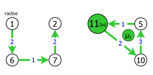
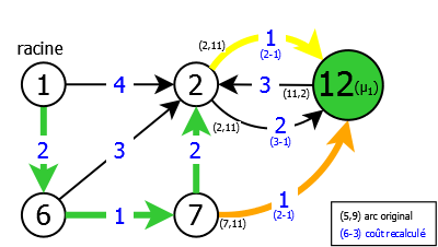
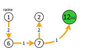
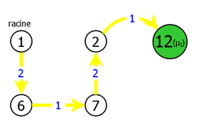
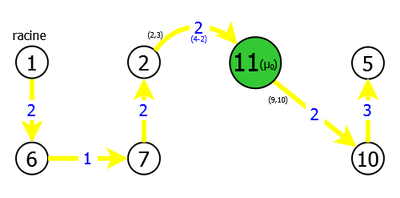
We then see there still are two components and a circuit μ₁ (5,11,10,5). So we will again contract the graph G₁ on the circuit μ₁ by replacing this latter by a pseudo-vertex 12. We then readjust the cost of the incoming arcs (2,11)(both of them) and (7,11) in μ₁, and finally relaunch the heuristic on the obtained graph G₂ = G₁/μ₁ = < S₂, A₂, C₂ >, which gives (see. figure 8):

Figure 8. The graph G₂ = < S₂, A₂, C₂ > and its two possible spanning subgraphs G'₂=< S₂, A'₂, C₂ >.

We then notice that the application of the heuristic on the graph G₂ can generate two distinct spanning subgraphs. Indeed, on the three incoming arcs to the pseudo-vertex 12, there are two of them with the same weight: the old arc (2,11) and the old arc (7,11), both entering in the circuit μ₁.

However, in both cases, the generated spanning subgraph G₂ is a tree T₂. So we only have to rebuild the MST T = T₀ of G = G₀ by successive recoveries of the trees T₁ and T₀, cas shown in figure 9:

Figure 9. Recovery of two possible MST of the graph G by successive rebuildings.

MSTs T1 (spanning subgraphs G'1) - recovery of μ1
MSTs T = T0 (spanning subgraphs G' = G'0) - recovery of μ0

We can therefore recover two different MSTs of the same weight equal to 20. Indeed, the two pairs of exchangeable arcs ((7,8),(4,3) and (2,3),(3,8)) have obviously the same cumulative weight which is in this case equal to 7 (5+2 or 4+3).

---

(Christophe "krisboul" Boullay)